2 loop 1 loop
play

2-loop 1-loop 0.4 0.3 0.2 V I N C I A R O O T 0.1 0 0 0.5 1 - PowerPoint PPT Presentation

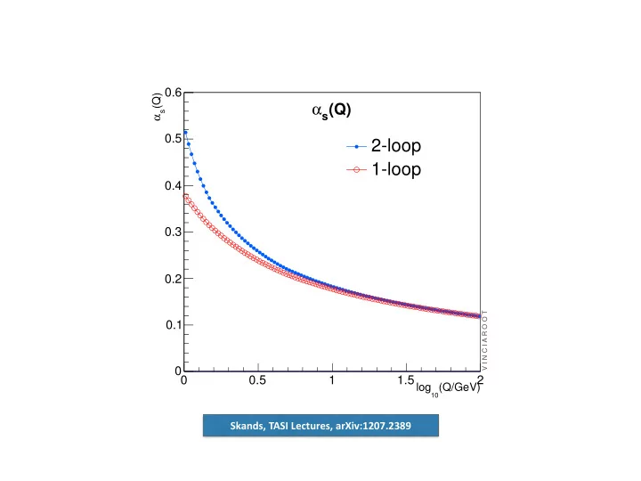
0.6 (Q) (Q) s s 0.5 2-loop 1-loop 0.4 0.3 0.2 V I N C I A R O O T 0.1 0 0 0.5 1 1.5 2 log (Q/GeV) 10 Skands, TASI Lectures, arXiv:1207.2389 Hartgring, Laenen, Skands, arXiv:1303.4974 Z 3


  1. 0.6 (Q) (Q) α s s α 0.5 2-loop 1-loop 0.4 0.3 0.2 V I N C I A R O O T 0.1 0 0 0.5 1 1.5 2 log (Q/GeV) 10 Skands, ¡TASI ¡Lectures, ¡arXiv:1207.2389

  2. Hartgring, ¡Laenen, ¡Skands, ¡arXiv:1303.4974 Z → 3 Jets i r y ij = s ij e w o h s M 2 Z Size of NLO “K” factor j y jk = s jk shower over phase space M 2 Z k Q E = 2 p T H strong L Q E = 2 p T H strong L 0 1.75 0 1.5 1.2 1.4 hard hard 1.2 - 2 - 2 1.5 collinear collinear 1.5 ln H y jk L ln H y jk L - 4 - 4 2 1.75 - 6 - 6 soft collinear soft collinear 1.75 1.2 - 8 - 8 - 8 - 6 - 4 - 2 0 - 8 - 6 - 4 - 2 0 ln H y ij L ln H y ij L (a) µ PS = √ s (b) µ PS = p ⊥

  3. Hartgring, ¡Laenen, ¡Skands, ¡arXiv:1303.4974 Z → 3 Jets Size of NLO “K” factor over phase space The “CMW” factor : Constant shift by 8 1 . 513 n F = 6 > α s β 0 > ✓ 67 − 3 π 2 − 10 n F / 3 > ◆ 1 . 569 n F = 5 < k 2 � � 2 ln ∼ 0 . 07 k CMW = exp = CMW 2(33 − 2 n F ) 1 . 618 n F = 4 2 π > > > 1 . 661 n F = 3 Catani, ¡Marchesini, ¡Webber, ¡NPB349 ¡(1991) ¡635 : Q E = 2 p T H strong L Q E = 2 p T H strong L 0 0 1.2 1.2 1.2 1.2 1.1 1.2 - 2 - 2 1.1 1.2 ln H y jk L ln H y jk L - 4 - 4 1.05 - 6 - 6 soft soft 1.2 1.1 - 8 - 8 - 8 - 6 - 4 - 2 0 - 8 - 6 - 4 - 2 0 ln H y ij L ln H y ij L µ PS = p ⊥ , with CMW (b) µ PS = p ⊥

  4. 0.8 (Q) α s (2) (MZ)=0.12 (incl var) α s 0.6 (2) (MZ)=0.12 (CMW) α s (1) (MZ)=0.14 α s 0.4 Beware : choosing a larger central scale → a seemingly smaller scale variation! 0.2 V I N C I A R O O T 0 1.2 1.1 Ratio 1 0.9 0.8 0 1 2 3 4 Log10( ) [GeV] µ 2 Loop: α s (M Z )=0.12 Λ 3 = 0.37 Λ 4 = 0.32 Λ 5 = 0.23 1 Loop: α s (M Z )=0.14 Λ 3 = 0.37 Λ 4 = 0.33 Λ 5 = 0.26 (In all cases, 5-flavor running is still used above mt)

  5. Variations in e + e - μ R by factor 2 in either direction Pythia 6 “Perugia 2012 : Variations” (with central choice μ R =p T , and α s (M Z ) (1) ~ 0.14) Skands, ¡ ¡arXiv:1005.3457 Thrust 3j 4j Durham kT Durham kT y 23 y 56 1-T 6-jet observable Event Shape 3-jet observable ∝ α s1 ∝ α s4 → Factor 2 looks Beware! α s pileup pretty extreme? See mcplots.cern.ch Karneyeu ¡et ¡al, ¡ ¡arXiv:1306.3436

  6. Variations in pp μ R by factor 2 in either direction Pythia 6 “Perugia 2012 : Variations” (with central choice μ R =p T , and α s (M Z ) (1) ~ 0.14) Skands, ¡ ¡arXiv:1005.3457 Z W Jets Jet p TZ p Tjet Shape d σ /dp T 1/ σ d σ /dp T → Factor 2 looks “dimensionful” “normalized” See mcplots.cern.ch reasonable? Karneyeu ¡et ¡al, ¡ ¡arXiv:1306.3436

  7. Cooper ¡et ¡al., ¡ ¡arXiv:1109.5295 Matrix Elements W+jets (E.g., AlpGen/MadGraph + Herwig/Pythia) jets) [pb] 4 10 pp, 7 TeV, W+jets, el-chan. P2011 PS , Alp. Λ ↑ Λ ↑ Λ PS ↓ , Λ Alp. ↓ jet Alp. Λ ↑ N Λ Alp. ↓ ≥ (W + 3 10 σ mcplots.cern.ch 2 10 Alpgen+Pythia jet multiplicity 0 1 2 3 N jet Ratio to 1.5 1 0.5 0 1 2 3 Jet Shape � Jet Shape � NJets PS ME+PS NJets: dominated by ME (+Sudakov from PS) Jet Shapes: dominated by PS

  8. From multi-leg LO to multi-leg NLO Hartgring, ¡Laenen, ¡Skands, ¡arXiv:1303.4974 ee hadrons → 91.2 GeV /d(1-T) 1-Thrust (udsc) 4 10 σ 2 /N d χ L3 bins 3 σ 10 5% 1/ (2) 0.5 0.0 ± (MZ)=0.12 (NLO3,CMW) α S 2 10 (1) 0.5 0.1 ± (MZ)=0.14 (LO3) α S 10 (2) 1.4 0.1 ± (MZ)=0.12 (LO3,CMW) α S (2) 15.0 0.6 ± (MZ)=0.12 (LO3) α 1 S -1 10 V I N C I A R O O T -2 10 Data from Phys.Rept. 399 (2004) 71 Vincia 1.104 + MadGraph 4.4.26 + Pythia 8.186 -3 10 1.2 Theory/Data 1.1 1 0.9 0.8 0 0.1 0.2 0.3 0.4 0.5 1-T (udsc)

  9. Multi-scale problems 0.005 W + 3 jets (100, 200, 300) 3 α s E.g., in context of ME 0.004 pT1 = 100 matching with many legs pT2 = 200 0.003 pT3 = 300 1 0.002 4 5 Example: W+3 3 0.001 V I N C I A R O O T 2 0.01 0 W + 3 jets (20, 30, 60) 2 3 α s 0.008 1.5 Ratio pT1 = 20 1 pT2 = 30 0.006 0.5 1 2 3 4 5 pT3 = 60 Central Choice 0.004 4 5 0.003 1 W' + 3 jets (100, 200, 300) 3 800 0.002 V I N C I A R O O T 2 3 α 0.0025 s mW = 800 0 pT1 = 100 0.002 2 pT2 = 200 4 1.5 5 0.0015 Ratio pT3 = 300 1 0.001 1 3 0.5 2 1 2 3 4 5 V I N C I A R O O T Central Choice 0.0005 1: MW � 0 2 2: MW + Sum(|pT|) � 3: -“- (quadratically) � 1.5 Ratio 4: Geometric mean pT (~PS) � 1 5: Arithmetic mean pT 0.5 1 2 3 4 5 Central Choice

Download Presentation
Download Policy: The content available on the website is offered to you 'AS IS' for your personal information and use only. It cannot be commercialized, licensed, or distributed on other websites without prior consent from the author. To download a presentation, simply click this link. If you encounter any difficulties during the download process, it's possible that the publisher has removed the file from their server.

Recommend


More recommend