15-11-2019 Department of Veterinary and Animal Sciences Linear - PDF document

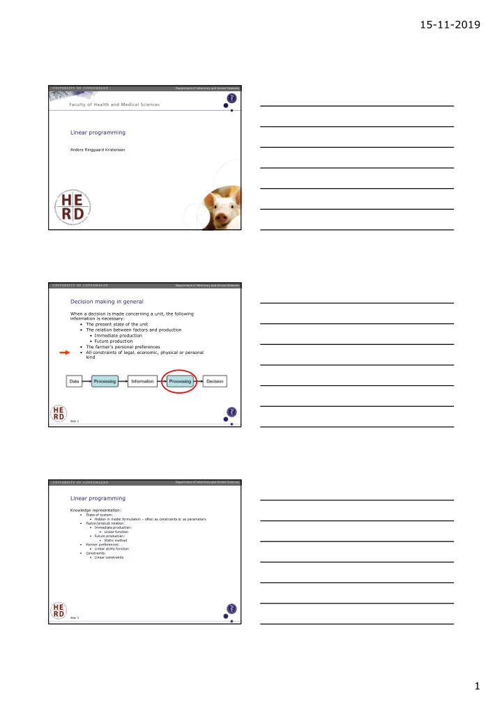
15-11-2019 Department of Veterinary and Animal Sciences Linear programming Anders Ringgaard Kristensen Department of Veterinary and Animal Sciences Decision making in general When a decision is made concerning a unit, the following information is necessary: • The present state of the unit • The relation between factors and production • Immediate production • Future production • The farmer’s personal preferences • All constraints of legal, economic, physical or personal kind Slide 2 Department of Veterinary and Animal Sciences Linear programming Knowledge representation: • State of system: • Hidden in model formulation – often as constraints or as parameters • Factor/product relation: • Immediate production: • Linear function • Future production: • Static method • Farmer preferences: • Linear utility function • Constraints: • Linear constraints Slide 3 1

15-11-2019 Department of Veterinary and Animal Sciences Example: Ration formulation A group of dairy cows is fed a ration consisting of x 1 kg silage and x 2 kg concentrates. The price of silage is p 1 and the price of concentrates is p 2 . The ration must satisfy some nutritional “demands”: • The energy content must be at least b 1 . The AAT 1 value must be at least b 2 • State of the cows The PBV 2 value must be at most b 3 • • The fill must be at most b 4 For both feeds, i , x i ≥ 0 Determine x 1 and x 2 so that the cost of the ration is minimized. 1 AAT = Amino Acids absorbed in the intestine 2 PBV = Protein balance in the rumen Slide 4 Department of Veterinary and Animal Sciences What are the states of the feeds? Energy (SFU/kg) of silage and concentrates: a 11 and a 12 , respectively. AAT (g/kg) of silage and concentrates: a 21 and a 22 , respectively. PBV (g/kg) of silage and concentrates: a 31 and a 32 , respectively. Fill (units/kg) of silage and concentrates: a 41 and a 42 , respectively. Slide 5 What are the states of the feeds? Silage Concentrates Energy a 11 a 12 AAT a 21 a 22 PBV a 31 a 32 Fill a 41 a 42 2

15-11-2019 Department of Veterinary and Animal Sciences LP problem Objective function p 1 x 1 + p 2 x 2 = Min! (minimize costs) - subject to a 11 x 1 + a 12 x 2 ≥ b 1 (energy at least b 1 ) a 21 x 1 + a 22 x 2 ≥ b 2 (AAT at least b 2 ) a 31 x 1 + a 32 x 2 ≤ b 3 (PBV at most b 3 ) a 41 x 1 + a 42 x 2 ≤ b 4 (fill at most b 4 ) x 1 ≥ 0, x 2 ≥ 0 Constraints Slide 7 Department of Veterinary and Animal Sciences The linear relations: Two “activities” a 11 x 1 + a 12 x 2 ≥ b 1 ⇔ x 2 x 2 ≥ b 1 / a 12 – ( a 11 / a 12 ) x 1 b 1 / a 12 The permitted area is bounded by a straight line in the diagram x 1 Slope: a 11 / a 12 Slide 8 Graphical solution, convex area x 2 Energy, ≥ AAT, ≥ PBV, ≤ Fill, ≤ The per-mitted area forms a convex set x 1 3

15-11-2019 Department of Veterinary and Animal Sciences The objective function p 1 x 1 + p 2 x 2 = c (costs) For fixed cost c’ we have x 2 = c’ / p 2 – ( p 1 / p 2 ) x 1 Combinations of x 1 and x 2 having same total cost form a straight line in the plane. Slide 10 Graphical solution, iso-cost line x 2 c’ / p 2 Combinations of x 1 and x 2 having cost c’ Slope: p 1 / p 2 We want to minimize cost c’ x 1 Graphical solution, minimization x 2 We want to minimize cost c’ Decrease c’ until the permitted area is reached. Decrease c’ until the lowest value of the permitted area is found. Optimal combination is x 1 ’, x 2 ’ x 2 ’ x 1 x 1 ’ 4

15-11-2019 Department of Veterinary and Animal Sciences What determines the optimum For a given set of constraints, the optimum is determined solely by the price relations. In our two-dimensional example it is simply the price ratio p 1 / p 2 Illustration Slide 13 Influence of prices, I x 2 Original setting x 2 ’ x 1 x 1 ’ Influence of prices, II x 2 Slight increase of p 1 Drastic change in terms of x 1 and x 2 but only sligtly in terms of costs c x 2 ’ x 1 x 1 ’ 5

15-11-2019 Influence of prices, III x 2 Large increase of p 2 Drastic change in terms of x 1 and x 2 and to some extent c x 2 ’ x 1 x 1 ’ Non-unique optimum x 2 Increase of p 2 All combinations of x 1 and x 2 along a border are optimal x 1 Department of Veterinary and Animal Sciences Properties of linear programming The permitted area is always a convex set The optimal solution is: • Either uniquely located in a corner • Or along a border line (accordingly also in two corners) It is therefore sufficient to search the corners of the convex set. A convex set A non-convex set Slide 18 6

15-11-2019 Department of Veterinary and Animal Sciences Modeling tricks From maximization to minimization: • p 1 x 1 + p 2 x 2 = Max! ⇔ - p 1 x 1 - p 2 x 2 = Min! From greater than to less than: • a i 1 x 1 + a i 2 x 2 ≥ b i ⇔ - a i 1 x 1 - a i 2 x 2 ≤ - b i From “equal to” to “less than” • a i 1 x 1 + a i 2 x 2 = b i ⇔ • - a i 1 x 1 - a i 2 x 2 ≤ - b i • a i 1 x 1 + a i 2 x 2 ≤ b i Slide 19 Department of Veterinary and Animal Sciences More than two variables We cannot illustrate graphically anymore, but the same principles apply: • Convex (multi-dimensional) set • Optimum always in a corner Slide 20 Department of Veterinary and Animal Sciences The simplex algorithm The most commonly applied optimization algorithm for linear programming. The simplex algorithm: • Identifies a corner of the convex set forming the permitted area. • Searches along the edges to find a better corner. • Checks whether the present corner is optimal Implemented in modern standard spreadsheets Implemented in ration formulation programs Slide 21 7

15-11-2019 Department of Veterinary and Animal Sciences Shadow prices What is the economic benefit of relaxing a constraint by one unit? • If it is not limiting it is zero! • Trivial method: • Change the constraint by one • Optimize again • How much did the result improve? • Software systems typically provides these values by default. Slide 22 Department of Veterinary and Animal Sciences Basic assumptions of LP Proportionality • No start-up costs • No decreasing returns to scale Additivity • No interactions between activities Divisibility • Any proportion of an activity allowed Certainty • All parameters (coefficients, prices, constraints) are known precisely. Slide 23 McCull and his sheep & steers McCull owns 200 ha of pasture where he can have ewes and/or Carrying capacity steers. Gross margins are $24 per ewe and Season Ewes Steers $60 per steer. Limited carrying capacity – refer to table Spring 15 5 Summer 24 4 Autumn 15 Winter 8 8

15-11-2019 McCull: LP-problem Objective function: 24 x 1 + 60 x 2 = Max! Constraints: 1/15 x 1 + 1/5 x 2 ≤ 200 Spring grazing 1/24 x 1 + 1/4 x 2 ≤ 200 Summer grazing x 1 ≤ 3000 (i.e 15 x 200) Sheep in autumn x 1 ≤ 1600 (i.e 8 x 200) Sheep in winter x 1 ≥ 0, x 2 ≥ 0 Department of Veterinary and Animal Sciences McCull: Graphical solution 5000 4500 4000 3500 3000 2500 2000 1500 1000 500 0 0 200 400 600 800 1000 Spring grazing Summer grazing Sheep in autumn Sheep in winter Iso-cost Slide 26 Department of Veterinary and Animal Sciences Properties of methods for decision support Herd constraints Optimization Linear programming Biological Functional variation limitations Slide 27 Uncertainty Dynamics 9