12 1 2019
play

12/1/2019 Department of Veterinary and Animal Sciences Advanced - PDF document

12/1/2019 Department of Veterinary and Animal Sciences Advanced Quantitative Methods in Herd Management The Normal Distribution and Confidence Intervals Leonardo de Knegt Anders Ringgaard Kristensen Department of Veterinary and Animal


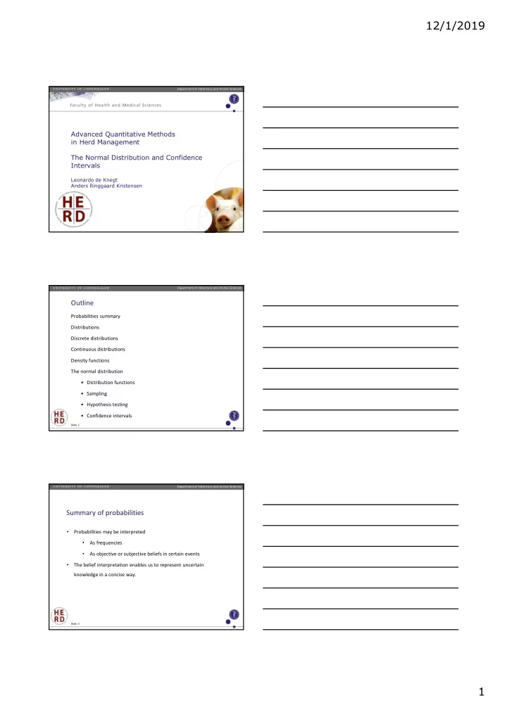
  1. 12/1/2019 Department of Veterinary and Animal Sciences Advanced Quantitative Methods in Herd Management The Normal Distribution and Confidence Intervals Leonardo de Knegt Anders Ringgaard Kristensen Department of Veterinary and Animal Sciences Outline Probabilities summary Distributions Discrete distributions Continuous distributions Density functions The normal distribution • Distribution functions • Sampling • Hypothesis testing • Confidence intervals Slide 2 Department of Veterinary and Animal Sciences Summary of probabilities • Probabilities may be interpreted • As frequencies • As objective or subjective beliefs in certain events • The belief interpretation enables us to represent uncertain knowledge in a concise way. Slide 3 1

  2. 12/1/2019 Department of Veterinary and Animal Sciences Distributions • In some cases the probability is defined by a certain function defined over the sample space. • In those cases, we say that the outcome is drawn from a standard distribution. • There exist standard distributions for many natural phenomena. • If the sample space is a countable set, we denote the corresponding distribution as discrete. Slide 4 Department of Veterinary and Animal Sciences Discrete distributions If X is the random variable representing the outcome, the expected value of a discrete distribution is defined as = 1 ∗ 1 6 + 2 ∗ 1 6 + 3 ∗ 1 6 + 4 ∗ 1 6 + 5 ∗ 1 6 + 6 ∗ 1 𝐹 𝑌 6 = 3.5 The variance is defined as 1 � + 2 � + 3 � + 4 � + 5 � + 6 � − 3.5 2 = 2.93 𝑊𝑏𝑠 𝑌 = 6 Slide 5 Department of Veterinary and Animal Sciences Continuous distributions • In some cases, the sample space S of a distribution is not countable. • If, furthermore, S is an interval on R, the random variable X taking values in S is said to have a continuous distribution. • For any x  S , we have P( X = x ) = 0. • Thus, no probability function exists for a continuous distribution can’t be expressed in tabular form. • Instead, the distribution is characterized by a density function f ( x ). Slide 6 2

  3. 12/1/2019 Department of Veterinary and Animal Sciences Density functions The density function f has the following properties (for a , b  R and a  b ) • • Thus, for a continuous distribution, f can only be interpreted as a probability when integrated over an interval. Slide 7 Department of Veterinary and Animal Sciences Continuous distributions For a continuous distribution, the expected value E( X ) is defined as And the variance is (just like the discrete case) Slide 8 Department of Veterinary and Animal Sciences The normal distribution • If S = R, and the random variable X has a normal distribution on S , then the density function is • The expected value and the variance simply turn out to be E( X ) =  , and Var( X ) =  2 We say that X is N(  ,  2 ), or X ~ N(  ,  2 ) • Slide 9 3

  4. 12/1/2019 Department of Veterinary and Animal Sciences The normal distribution • The normal distribution may be used to represent almost all kinds of random outcome on the continuous scale in the real world. • Exceptions: phenomena that are bounded in some sense (e.g. the waiting time to be served in a queue cannot be negative) • It can be showed (central limit theorems) that if X 1 , X 2 , …, X n are random variables of (more or less) any kind, then the sum Y n = X 1 + X 2 + …+ X n is normally distributed for n sufficiently large. • The normal distribution is the cornerstone among statistical distributions. Slide 10 Department of Veterinary and Animal Sciences Normal distributions Three normal distributions 0,5 0,4 m=0, s=3 0,3 f( x ) m=-5, s=1 0,2 m=0, s=1 0,1 0 -10 -5 0 5 10 x Three normal distributions with mean m and standard deviation s Slide 11 Department of Veterinary and Animal Sciences Normal distributions • The normal distribution with  = 0, and  = 1 is called the standard normal distribution. • A random variable being standard normally distributed is often denoted as Z • The density function of the standard normal distribution is often denoted as  (phi) . It follows that Slide 12 4

  5. 12/1/2019 Department of Veterinary and Animal Sciences Normal distributions: operation properties Let X 1 ~ N(  1 ,  1 2 ), X 2 ~ N(  2 ,  2 • 2 ), and X 1 and X 2 are independent. • Define Y 1 = X 1 + X 2 and Y 2 = X 1 − X 2 . Then • Y 1 ~ N(  1 +  2 ,  1 2 +  2 2 ) • Y 2 ~ N(  1 −  2 ,  1 2 +  2 2 ) • Let a and b be arbitrary real numbers, and let X ~ N(  ,  2 ). • Define Y = aX + b . Then, Y ~ N( a  + b, a 2  2 ) Slide 13 Department of Veterinary and Animal Sciences Normal distributions From the previous slide it follows in particular, that if X ~ N(  ,  2 ), then • So, if f is the density function of X ~ N(  ,  2 ), then • Thus, we can calculate the value of any density function for a normal distribution from the density distribution of the standard normal distribution. Slide 14 Department of Veterinary and Animal Sciences Distribution functions • We have so far defined distributions by: • probability functions (discrete distributions) • density functions (continuous distributions). • We might just as well have used the distribution function F , which is defined in the same way for both classes of distributions: • F ( x ) = P( X  x ) • F(x) is called the distribution function, or the Cumulative Distribution Function (CDF) Slide 15 5

  6. 12/1/2019 Department of Veterinary and Animal Sciences Distribution functions Even though the definition is the same, the value of the distribution function is calculated in different ways for the two classes of distributions. • For discrete distributions • For continuous distributions Slide 16 Department of Veterinary and Animal Sciences Distribution functions Recap: • F(X): Cumulative Distribution Function of X • F(x) = P(X ≤ x) • probability that the random variable X takes a value smaller than some specific value x • f(x): Probability Density Function of x • • Probability that the random variable x takes a value within an interval Slide 17 Department of Veterinary and Animal Sciences Distribution functions • From the formula above, it follows directly that for a continuous distribution, F ’( x ) = f ( x ) • The distribution function of the standard normal distribution is often denoted as  , and naturally  ’( z ) =  ( z ) . No closed form (formula) exists for  , it must be looked up in tables. Slide 18 6

  7. 12/1/2019 Department of Veterinary and Animal Sciences Distribution functions Any distribution function F has the following two properties: • F ( x )  0 for x  -  • F ( x )  1 for x   Three normal distributions Three normal distributions 0,5 1 0,4 0,8 m=0, s=3 m=0, s=3 0,3 0,6 f( x ) f( x ) m=-5, s=1 m=-5, s=1 0,2 0,4 m=0, s=1 m=0, s=1 0,1 0,2 0 0 -10 -5 0 5 10 -10 -5 0 5 10 x x Density function Distribution function Slide 19 Department of Veterinary and Animal Sciences Sampling form a distribution Assume that X 1 , X 2 , …, X n are sampled independently from the same distribution having the known expectation  and the known standard deviation  Then the mean of the sample has the expected value  and the standard deviation In particular, if the X i ’s are N(  ,  2 ) then the sample mean is N(  ,  2 / n ) Slide 20 Department of Veterinary and Animal Sciences Sampling from a Normal Distribution • Assume that X 1 , X 2 , …, X n are sampled independently from the same normal distribution N(  ,  2 ) where  is unknown and  is known. • For some reason we expect (hope) that  has a certain value  0 , and we would therefore like to test the following hypothesis: H 0 :  =  0 • How can we do that? Well, we know that the sample mean is N(  ,  2 / n ) Slide 21 7

  8. 12/1/2019 Hypothesis testing in normal distributions A normal distribution with standard deviation 3 A normal distribution with standard deviation 3 0,2 1 0,8 0,6 f( x ) 0,1 m=0, s=3 f( x ) m=0, s=3 0,4 0,2 0 0 -1 -9 -8 -7 -6 -5 -4 -3 -2 -1 0 1 2 3 4 5 6 7 8 9 10 -1 -9 -8 -7 -6 -5 -4 -3 -2 -1 0 1 2 3 4 5 6 7 8 9 10 0 0 x x • Observations close to the mean are far more likely than distant observations. • From the distribution function we can calculate the likelihood that an observation falls within the interval  ±  Hypothesis testing in normal distributions 𝑎 = 𝑌 − 𝜈 For a standard normal distribution (z): 𝜏 𝑔(𝑦) = ฀( ��� � ) …which that translates to our density function: Phi is the area For the interval  ±  , where  = 0,  =1 • under the curve! P (𝜈 −   𝑌  𝜈 +  ) =  (𝜈 +  ) -  (𝜈 −  ) F(x) = P(X ≤ x) Always gives the area to the left -  0  Hypothesis testing in normal distributions P (𝜈 −   𝑌  𝜈 +  ) =  (𝜈 +  ) -  (𝜈 −  ) P (0 − 1  𝑌  0 + 1) =  (0 + 1 ) −  (0 − 1 ) P (−1  𝑌  1) =  (1 ) -  (−1 ) Look up at the z table! 8

Download Presentation
Download Policy: The content available on the website is offered to you 'AS IS' for your personal information and use only. It cannot be commercialized, licensed, or distributed on other websites without prior consent from the author. To download a presentation, simply click this link. If you encounter any difficulties during the download process, it's possible that the publisher has removed the file from their server.

Recommend


More recommend