10/12/2019 Definitions A schedule is said to be feasible if it - PDF document

10/12/2019 Definitions A schedule  is said to be feasible if it satisfies a set of constraints. A task set  is said to be feasible , if there exists an algorithm that generates a feasible schedule for  . A task set  is said to be schedulable with an algorithm A, if A generates a feasible schedule. Examples of constraints • Timing constraints: activation, period, deadline, jitter. • Precedence: order of execution between tasks. • Resources: synchronization for mutual exclusion. 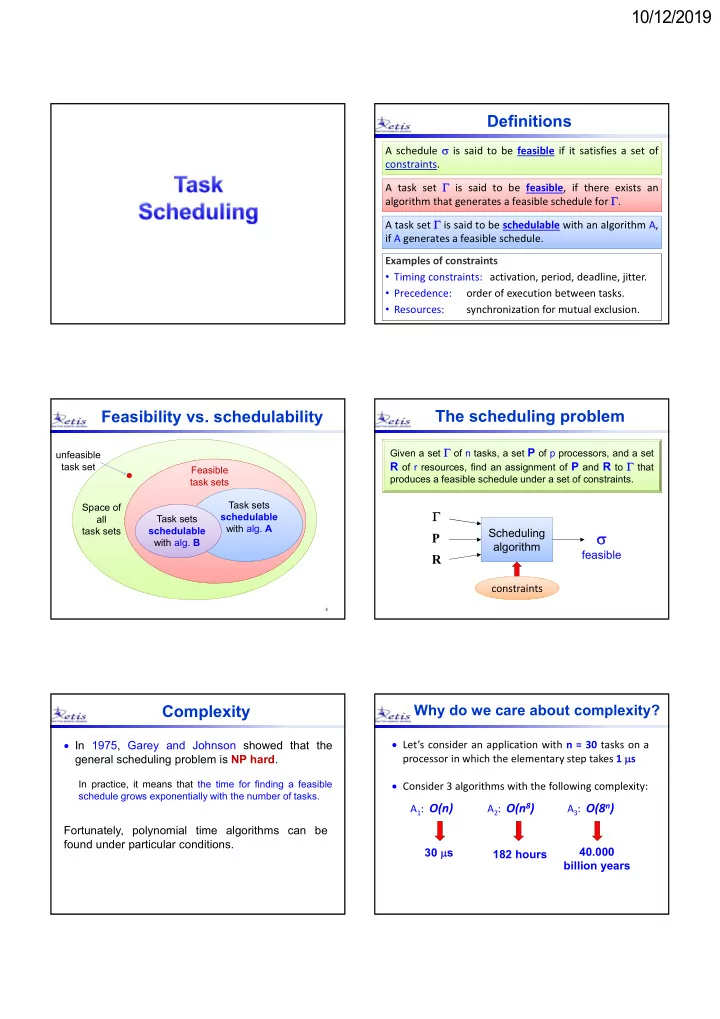Feasibility vs. schedulability The scheduling problem Given a set  of n tasks, a set P of p processors, and a set unfeasible R of r resources, find an assignment of P and R to  that task set Feasible produces a feasible schedule under a set of constraints. task sets Task sets Space of  schedulable all Task sets with alg. A task sets schedulable Scheduling  P with alg. B algorithm feasible R constraints 3 Complexity Why do we care about complexity?  In 1975, Garey and Johnson showed that the  Let’s consider an application with n = 30 tasks on a processor in which the elementary step takes 1  s general scheduling problem is NP hard . In practice, it means that the time for finding a feasible  Consider 3 algorithms with the following complexity: schedule grows exponentially with the number of tasks. A 2 : O(n 8 ) A 3 : O(8 n ) A 1 : O(n) Fortunately, polynomial time algorithms can be found under particular conditions. 30  s 40.000 182 hours billion years

10/12/2019 Simplifying assumptions Algorithm taxonomy  Single processor  Preemptive vs. Non Preemptive  Homogeneous task sets  Static vs. dynamic  Fully preemptive tasks  On line vs. Off line  Simultaneous activations  No precedence constraints  Optimal vs. Heuristic  No resource constraints Static vs. Dynamic Off-line vs. On-line Static Off-line scheduling decisions are taken based on all scheduling decisions are taken before fixed parameters, statically assigned to task activation: the schedule is stored in a tasks before activation. table ( table-driven scheduling ). Dynamic On-line scheduling decisions are taken based on scheduling decisions are taken at run time parameters that can change with time. on the set of active tasks. Optimal vs. Heuristic Optimality criteria Optimal  Feasibility : Find a feasible schedule if there They generate a schedule that minimizes exists one. a cost function, defined based on an optimality criterion.  Minimize the maximum lateness  Minimize the number of deadline miss Heuristic They generate a schedule according to a  Assign a value to each task, then maximize heuristic function that tries to satisfy an the cumulative value of the feasible tasks optimality criterion, but there is no guarantee of success.

10/12/2019 Task set assumptions Graham’s Notation We consider algorithms for different types of tasks:  denotes the number of processors      Single-job tasks (one shot) denotes the constraints on tasks  tasks with a single activation (not recurrent) denotes the optimality criterion  Periodic tasks Examples: recurrent tasks regularly activated by a timer (each task potentially generates infinite jobs) preem. R avg 1 Uniprocessor algorithm for preemptive tasks that minimizes the average response time.  Aperiodic/Sporadic tasks Dual-core algorithm for synchronous tasks that 2 sync L max recurrent tasks irregularly activated by events (each minimizes the maximum lateness. task potentially generates infinite jobs) preem. L max 4 Quad-core algorithm for preemptive tasks that  Mixed task sets minimizes the maximum lateness. Classical scheduling policies First Come First Served It assigns the CPU to tasks based on their arrival  First Come First Served times (intrinsically non preemptive):  Shortest Job First Ready queue  Priority Scheduling  4  3  2  1 CPU  Round Robin   1  2  3  4 Not suited for real-time systems t a 1 a 2 a 3 a 4 s 2 s 3 s 4 f 4 First Come First Served Shortest Job First (SJF) ‐ Very unpredictable It selects the ready task with the shortest response times strongly depend on task arrivals: computation time. a 1 a 2 a 3  Static (C i is a constant parameter) R 1 = 20 R 2 = 26 R 3 = 26  2  3  1 t  It can be used on line or off‐line 0 4 8 12 16 20 24 28 32 a 3 a 2 a 1  Can be preemptive or non preemptive R 1 = 26 R 2 = 8 R 3 = 2  3  2  1  It minimizes the average response time t 0 4 8 12 16 20 24 28 32 17 18

10/12/2019 SJF - Optimality SJF - Optimality  SJF  L S   ’  ’’  * . . .  ’ . . .       R (  R ( ) R ( ') R ( ' ' ) *) S L t r 0 f S ’ < f L f L ’ = f S  * =  SJF f S ’ + f L ’  f S + f L R  ( ) is the minimum response time SJF n n 1 1 achievable by any algorithm          R ( ') ( f ' r ) ( f r ) R ( ) i i i i n n   i 1 i 1 19 20 Priority Scheduling Is SJF suited for Real-Time?  Each task has a priority P i , typically P i  [0, 255] ‐ It is not optimal in the sense of feasibility  The task with the highest priority is selected for d 1 d 2 d 3 A  SJF feasible execution.  2  3  1  Tasks with the same priority are served FCFS t 0 4 8 12 16 20 24 28 32 d 1 d 2 d 3 SJF not feasible p i  1/C i  SJF NOTE:  3  2  1 p i  1/a i  FCFS t 0 4 8 12 16 20 24 28 32 21 22 Priority Scheduling Round Robin The ready queue is served with FCFS, but ...  Problem: starvation ‐ Each task  i cannot execute for more than Q low priority tasks may experience long delays due to the preemption of high priority tasks. time units (Q = time quantum). ‐ When Q expires,  i is put back in the queue.  A possible solution: aging READY queue priority increases with waiting time CPU Q expired 23 24

10/12/2019 Round Robin Round Robin n = number of task in the system ‐ if Q > max(C i ) then RR  FCFS nQ nQ ‐ if Q  context switch time (  ) then n(Q +  ) n(Q +  ) t C Q   R ( nQ ) i nC t i i Q Q +  Time sharing     C Q       R n ( Q ) i nC   Each task runs as it was executing alone on a virtual i i Q Q   processor n times slower than the real one. 25 26 Multi-Level Scheduling Multi-Level Scheduling system tasks High priority PRIORITY priority CPU interactive tasks RR CPU Medium priority batch tasks Low priority FCFS 27 28 Real-Time Algorithms They can either schedule tasks by  relative deadlines D i ( static )  absolute deadlines d i ( dynamic ) D i r i d i 30

10/12/2019 Earliest Due Date Lateness Problem 1 sync L max L i = f i  d i Algorithm [Jackson 55] L i > 0 - Order the ready queue by increasing deadline. Assumptions - All the tasks are simultaneously activated r i f i d i - Preemption is not needed. L i < 0 - Static (D i is fixed) Property f i d i r i - It minimizes the maximum lateness (L max ) 31 32 Maximum Lateness EDD - Optimality  EDD  L max = max i (L i ) B A  ’ A B t r 0 f a ’ < f b f b ’ = f a d a d b L max = L a = f a  d a if (L max < 0) then L a ’ = f a ’  d a < f a  d a no task exceeds its deadline L’ max < L max L b ’ = f b ’  d b < f a  d a 33 34 EDD guarantee test (off line) EDD - Optimality   ’  ’’  * . . .  1  2  3  4 t       L max  L ( ) L ( ') L ( ' ' ) . . . ( *) f 1 f 2 f 3 f 4 max max max   A task set  is feasible iff i f d  * =  EDD i i  L ( ) i   i is the minimum value   max EDD f C  i C D achievable by any algorithm i k k i  k 1  1 k 35 36

10/12/2019 Earliest Deadline First EDF Example preem. L max Problem 1 Algorithm [Horn 74] - Order the ready queue by increasing absolute deadline Assumptions - Tasks can be activated dynamically - Dynamic algorithm ( d i depends on a i ) - Tasks can be preempted at any time Property - It minimizes the maximum lateness (L max ) 37 38 EDF Guarantee test (on line) Complexity c 1 (t) EDD O(n logn) Scheduler (queue ordering): c 2 (t) O(n) Feasibility Test (guarantee test): c 3 (t) EDF c 4 (t) O(n) Scheduler (insertion in the queue): Feasibility Test (guarantee single task): O(n) t   i   i c ( t ) d t k i  1 k 39 40 EDF optimality Dertouzos Transformation for ( t = 0 to D max –1)  (t) = task executing at time t  In the sense of feasibility [Dertouzos 1974] if (  (t)  E(t) ) { E(t) = task with min d at time t  (t E ) =  (t) ; t E = time at which E is executed  (t) = E(t) ; An algorithm A is optimal in the sense of }    EDF feasibility if it generates a feasible schedule, if  1 there exists one.  2  3 Demonstration method  4 It is sufficient to prove that, given an arbitrary 0 2 4 6 8 10 12 14 16 feasible schedule, the schedule generated by  (t) = 4 EDF is also feasible. E(t) = 2 t = 4 t E = 6 41 42