1 Modeling Assumptions The Dangers of Optimism and Pessimism - PDF document

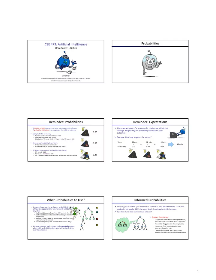
Probabilities CSE 473: Artificial Intelligence Uncertainty, Utilities Dieter Fox [These slides were created by Dan Klein and Pieter Abbeel for CS188 Intro to AI at UC Berkeley. All CS188 materials are available at http://ai.berkeley.edu.] Reminder: Probabilities Reminder: Expectations § A random variable represents an event whose outcome is unknown § The expected value of a function of a random variable is the A probability distribution is an assignment of weights to outcomes § average, weighted by the probability distribution over 0.25 outcomes Example: Traffic on freeway § § Random variable: T = whether there’s traffic § Example: How long to get to the airport? § Outcomes: T in {none, light, heavy} § Distribution: P(T=none) = 0.25, P(T=light) = 0.50, P(T=heavy) = 0.25 Time: 20 min 30 min 60 min 0.50 § Some laws of probability (more later): + + 35 min x x x § Probabilities are always non-negative Probability: 0.25 0.50 0.25 § Probabilities over all possible outcomes sum to one § As we get more evidence, probabilities may change: § P(T=heavy) = 0.25, § P(T=heavy | Hour=8am) = 0.60 0.25 § We’ll talk about methods for reasoning and updating probabilities later What Probabilities to Use? Informed Probabilities § Let’s say you know that your opponent is sometimes lazy. 20% of the time, she moves § In expectimax search, we have a probabilistic model of how the opponent (or environment) will behave in randomly, but usually (80%) she runs a depth 2 minimax to decide her move any state § Question: What tree search should you use? § Model could be a simple uniform distribution (roll a die) § Model could be sophisticated and require a great deal of computation § Answer: Expectimax! § We have a chance node for any outcome out of our control: § To figure out EACH chance node’s probabilities, opponent or environment you have to run a simulation of your opponent § The model might say that adversarial actions are likely! 0.1 0.9 § This kind of thing gets very slow very quickly § For now, assume each chance node magically comes Even worse if you have to simulate your § along with probabilities that specify the distribution opponent simulating you… over its outcomes … except for minimax, which has the nice § property that it all collapses into one game tree 1

Modeling Assumptions The Dangers of Optimism and Pessimism Dangerous Optimism Dangerous Pessimism Assuming chance when the world is adversarial Assuming the worst case when it’s not likely Video of Demo World Assumptions Video of Demo World Assumptions Random Ghost – Expectimax Pacman Adversarial Ghost – Minimax Pacman Video of Demo World Assumptions Video of Demo World Assumptions Adversarial Ghost – Expectimax Pacman Random Ghost – Minimax Pacman 2

Assumptions vs. Reality Other Game Types Adversarial Ghost Random Ghost Won 5/5 Won 5/5 Minimax Pacman Avg. Score: 483 Avg. Score: 493 Won 1/5 Won 5/5 Expectimax Pacman Avg. Score: -303 Avg. Score: 503 Results from playing 5 games Pacman used depth 4 search with an eval function that avoids trouble Ghost used depth 2 search with an eval function that seeks Pacman Example: Backgammon Mixed Layer Types § E.g. Backgammon § Expectiminimax § Environment is an extra “random agent” player that moves after each min/max agent § Each node computes the appropriate combination of its children Image: Wikipedia Example: Backgammon Different Types of Ghosts? § Dice rolls increase b : 21 possible rolls with 2 dice § Backgammon ~ 20 legal moves § Depth 2 = 20 x (21 x 20) 3 = 1.2 x 10 9 Stupid § As depth increases, probability of reaching a given search node shrinks Devilish Smart § So usefulness of search is diminished § So limiting depth is less damaging § But pruning is trickier… § Historic AI (1992): TDGammon uses depth-2 search + very good evaluation function + reinforcement learning: world-champion level play § 1 st AI world champion in any game! Image: Wikipedia 3

Multi-Agent Utilities Utilities § What if the game is not zero-sum, or has multiple players? § Generalization of minimax: § Terminals have utility tuples § Node values are also utility tuples § Each player maximizes its own component § Can give rise to cooperation and competition dynamically… 1,6,6 7,1,2 6,1,2 7,2,1 5,1,7 1,5,2 7,7,1 5,2,5 Maximum Expected Utility What Utilities to Use? § Why should we average utilities? § Principle of maximum expected utility: § A rational agent should chose the action that maximizes its expected utility, 20 30 x 2 400 900 0 40 0 1600 given its knowledge § Questions: § For worst-case minimax reasoning, terminal function scale doesn’t matter § We just want better states to have higher evaluations (get the ordering right) § Where do utilities come from? § We call this insensitivity to monotonic transformations § How do we know such utilities even exist? § How do we know that averaging even makes sense? § For average-case expectimax reasoning, we need magnitudes to be meaningful § What if our behavior (preferences) can’t be described by utilities? Utilities Utilities: Uncertain Outcomes Getting ice cream § Utilities are functions from outcomes (states of the world) to real numbers that describe an agent’s preferences Get Single Get Double § Where do utilities come from? § In a game, may be simple (+1/-1) § Utilities summarize the agent’s goals Oops Whew! § Theorem: any “rational” preferences can be summarized as a utility function § We hard-wire utilities and let behaviors emerge § Why don’t we let agents pick utilities? § Why don’t we prescribe behaviors? 4

Preferences Rationality A Prize A Lottery § An agent must have preferences among: § Prizes: A, B , etc. A § Lotteries: situations with uncertain prizes p 1 -p A B § Notation: § Preference: § Indifference: Rational Preferences Rational Preferences The Axioms of Rationality § We want some constraints on preferences before we call them rational, such as: Ù Þ Axiom of Transitivity: ( A ! B ) ( B ! C ) ( A ! C ) § For example: an agent with intransitive preferences can be induced to give away all of its money § If B > C, then an agent with C would pay (say) 1 cent to get B § If A > B, then an agent with B would pay (say) 1 cent to get A § If C > A, then an agent with A would pay (say) 1 cent to get C Theorem: Rational preferences imply behavior describable as maximization of expected utility MEU Principle Human Utilities § Theorem [Ramsey, 1931; von Neumann & Morgenstern, 1944] § Given any preferences satisfying these constraints, there exists a real-valued function U such that: § I.e. values assigned by U preserve preferences of both prizes and lotteries! § Maximum expected utility (MEU) principle: § Choose the action that maximizes expected utility § Note: an agent can be entirely rational (consistent with MEU) without ever representing or manipulating utilities and probabilities § E.g., a lookup table for perfect tic-tac-toe, a reflex vacuum cleaner 5

Utility Scales Human Utilities § Utilities map states to real numbers. Which numbers? § Normalized utilities: u + = 1.0, u - = 0.0 § Standard approach to assessment (elicitation) of human utilities: § Micromorts: one-millionth chance of death, useful for § Compare a prize A to a standard lottery L p between paying to reduce product risks, etc. § “best possible prize” u + with probability p § QALYs: quality-adjusted life years, useful for medical § “worst possible catastrophe” u - with probability 1-p decisions involving substantial risk § Adjust lottery probability p until indifference: A ~ L p § Resulting p is a utility in [0,1] § Note: behavior is invariant under positive linear transformation 0.999999 0.000001 Pay $30 § With deterministic prizes only (no lottery choices), only No change Instant death ordinal utility can be determined, i.e., total order on prizes Money Example: Insurance § Money does not behave as a utility function, but we can talk about the § Consider the lottery [0.5, $1000; 0.5, $0] utility of having money (or being in debt) § What is its expected monetary value? ($500) § Given a lottery L = [p, $X; (1-p), $Y] § What is its certainty equivalent? § The expected monetary value EMV(L) is p*X + (1-p)*Y § Monetary value acceptable in lieu of lottery § U(L) = p*U($X) + (1-p)*U($Y) § $400 for most people § Typically, U(L) < U( EMV(L) ) § Difference of $100 is the insurance premium § In this sense, people are risk-averse § There’s an insurance industry because people § When deep in debt, people are risk-prone will pay to reduce their risk § If everyone were risk-neutral, no insurance needed! § It’s win-win: you’d rather have the $400 and the insurance company would rather have the lottery (their utility curve is flat and they have many lotteries) Example: Human Rationality? Kahneman & Tversky Choose between § Famous example of Allais (1953) Option A Option B § A: [0.8, $4k; 0.2, $0] § 33% $2500 § 100% $2400 § B: [1.0, $3k; 0.0, $0] § 66% $2400 § C: [0.2, $4k; 0.8, $0] § 01% 0 § D: [0.25, $3k; 0.75, $0] [18] [82]* § Most people prefer B > A, C > D § But if U($0) = 0, then § B > A è U($3k) > 0.8 U($4k) § C > D è 0.8 U($4k) > U($3k) 6