1 Growth in Performance of RAM & CPU Technology Trends - - PDF document

1 CSE775: Computer Architecture

1

Chapter 1: Fundamentals of Computer Design

Computer Architecture Topics

DRAM Disks, WORM, Tape Coherence, Emerging Technologies Interleaving Memories RAID Input/Output and Storage

2 Instruction Set Architecture

Pipelining, Hazard Resolution, Superscalar, Reordering, Prediction, Speculation, Vector, DSP Addressing, Protection, Exception Handling L1 Cache L2 Cache Coherence, Bandwidth, Latency VLSI Memory Hierarchy Pipelining and Instruction Level Parallelism

Computer Architecture Topics

M Interconnection Network S P M P M P M P ° ° °

Network Interfaces Shared Memory, Message Passing, Data Parallelism

3

Topologies, Routing, Bandwidth, Latency, Reliability

Processor-Memory-Switch

Multiprocessors Networks and Interconnections

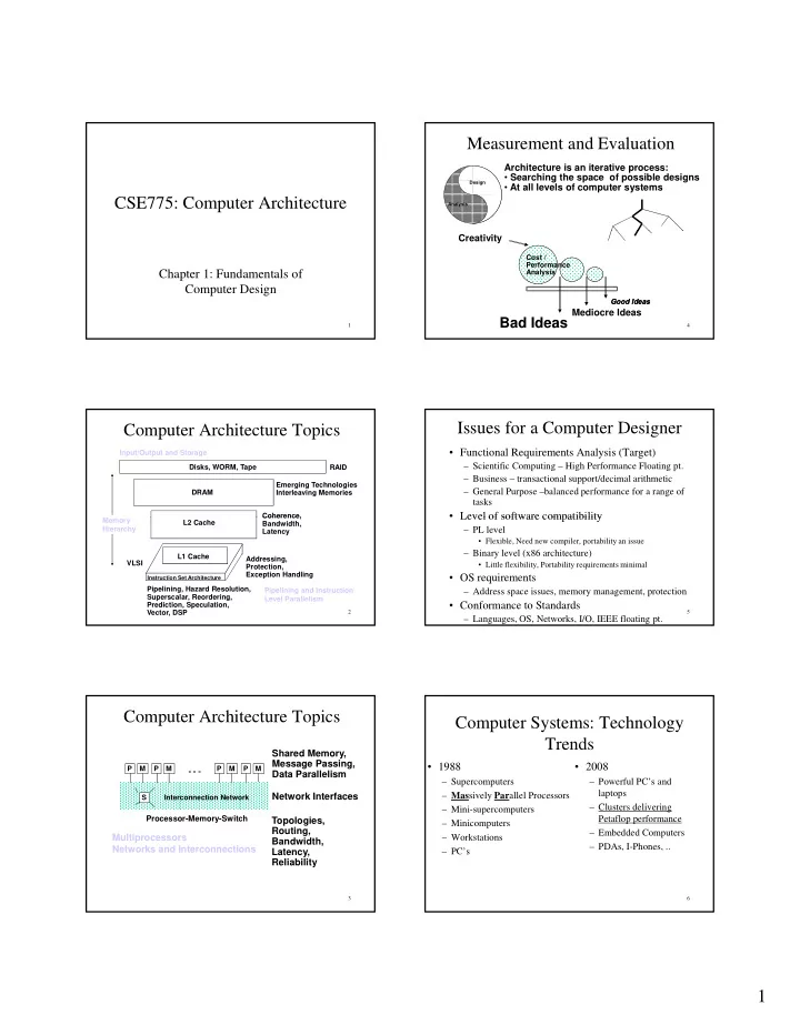
Measurement and Evaluation

Design Analysis

Architecture is an iterative process:

• Searching the space of possible designs
• At all levels of computer systems

4

Creativity

Good Ideas Good Ideas

Mediocre Ideas

Bad Ideas

Cost / Performance Analysis

Issues for a Computer Designer

• Functional Requirements Analysis (Target)

– Scientific Computing – High Performance Floating pt. – Business – transactional support/decimal arithmetic – General Purpose –balanced performance for a range of tasks

• Level of software compatibility

5

Level of software compatibility

– PL level

• Flexible, Need new compiler, portability an issue

– Binary level (x86 architecture)

• Little flexibility, Portability requirements minimal
• OS requirements

– Address space issues, memory management, protection

• Conformance to Standards

– Languages, OS, Networks, I/O, IEEE floating pt.

Computer Systems: Technology Trends

• 1988

– Supercomputers – Massively Parallel Processors

• 2008

– Powerful PC’s and laptops Cl d li i

6

– Mini-supercomputers – Minicomputers – Workstations – PC’s – Clusters delivering Petaflop performance – Embedded Computers – PDAs, I-Phones, ..

2 Technology Trends

• Integrated circuit logic technology – a growth in transistor

count on chip of about 40% to 55% per year.

• Semiconductor RAM – capacity increases by 40% per

year, while cycle time has improved very slowly, decreasing by about one-third in 10 years. Cost has decreased at rate about the rate at which capacity increases.

7

• Magnetic disc technology – in 1990’s disk density had been

improving 60% to100% per year, while prior to 1990 about 30% per year. Since 2004, it dropped back to 30% per year.

• Network technology – Latency and bandwidth are important.

Internet infrastructure in the U.S. has been doubling in bandwidth every year. High performance Systems Area Network (such as InfiniBand) delivering continuous reduced latency.

Why Such Change in 20 years?

• Performance

– Technology Advances

• CMOS (complementary metal oxide semiconductor) VLSI

dominates older technologies like TTL (Transistor Transistor Logic) in cost AND performance

– Computer architecture advances improves low-end

• RISC, pipelining, superscalar, RAID, …

8

, p p g, p , ,

• Price: Lower costs due to …

– Simpler development

• CMOS VLSI: smaller systems, fewer components

– Higher volumes – Lower margins by class of computer, due to fewer services

Growth in Microprocessor Performance

Figure 1.1

9

In 90’s, the main source of innovations in computer design has come from RISC-style pipelined processors. In the last several years, the annual growth rate is (only) 10-20%.

Growth in Performance of RAM & CPU

Figure 5.2

10

• Mismatch between CPU performance growth and memory performance growth!!
• And, almost unchanged memory latency
• Little instruction-level parallelism left to exploit efficiently
• Maximum power dissipation of air-cooled chips reached

Cost of Six Generations of DRAMs

11

Cost of Microprocessors

12

3 Components of Price for a $1000 PC

13

IC cost = Die cost + Testing cost + Packaging cost Final test yield Die cost = Wafer cost Dies per Wafer * Die yield Dies per wafer = š * ( Wafer_diam / 2)2 – š * Wafer_diam – Test dies Die Area ¦ 2 * Die Area

Integrated Circuits Costs

14

DAP.S98 1

Die Area ¦ 2 Die Area Die Yield = Wafer yield * 1 + Defects_per_unit_area * Die_Area

α

Die Cost goes roughly with die area4

{

− α

}

Failures and Dependability

• Failures at any level costs money

– Integrated circuits (processor, memory) – Disks – Networks

• Costs Millions of Dollars for 1hour downtime

15

• Costs Millions of Dollars for 1hour downtime

(Amazon, Google, ..)

• No concept of downtime at the middle of night
• Systems need to be designed with fault-

tolerance

– Hardware – Software

Performance and Cost

Plane Boeing 747 Speed 610 mph DC to Paris 6.5 hours Passengers 470 Throughput (pmph) 286,700

16

• Time to run the task (ExTime)

– Execution time, response time, latency

• Tasks per day, hour, week, sec, ns … (Performance)

– Throughput, bandwidth BAD/Sud Concodre 1350 mph 3 hours 132 178,200

The Bottom Line: Performance (and Cost)

"X is n times faster than Y" means ExTime(Y) Performance(X)

• =
• 17

ExTime(X) Performance(Y)

• Speed of Concorde vs. Boeing 747
• Throughput of Boeing 747 vs. Concorde

Metrics of Performance

Compiler Programming Language Application Answers per month Operations per second

18

Datapath Control Transistors Wires Pins

ISA

Function Units (millions) of Instructions per second: MIPS (millions) of (FP) operations per second: MFLOP/s Cycles per second (clock rate) Megabytes per second

4 Computer Engineering Methodology

Evaluate Existing Evaluate Existing Systems for Systems for Bottlenecks Bottlenecks Benchmarks Implementation Complexity

19

Simulate New Simulate New Designs and Designs and Organizations Organizations Implement Next Implement Next Generation System Generation System

Technology Trends

Benchmarks Workloads

Measurement Tools

• Benchmarks, Traces, Mixes
• Hardware: Cost, delay, area, power estimation
• Simulation (many levels)

– ISA, RT, Gate, Circuit

Q i Th

20

• Queuing Theory
• Rules of Thumb
• Fundamental “Laws”/Principles
• Understanding the limitations of any

measurement tool is crucial.

Issues with Benchmark Engineering

• Motivated by the bottom dollar, good

performance on classic suites more customers, better sales.

21

,

• Benchmark Engineering Limits the

longevity of benchmark suites

• Technology and Applications Limits the

longevity of benchmark suites.

SPEC: System Performance Evaluation Cooperative

• First Round 1989

– 10 programs yielding a single number (“SPECmarks”)

• Second Round 1992

– SPECInt92 (6 integer programs) and SPECfp92 (14 floating point programs)

22

g p p g ) – “benchmarks useful for 3 years”

• SPEC CPU2000 (11 integer benchmarks – CINT2000, and

14 floating-point benchmarks – CFP2000

• SPEC 2006 (CINT2006, CFP2006)
• Server Benchmarks

– SPECWeb – SPECFS

• TPC (TPA-A, TPC-C, TPC-H, TPC-W, …)

SPEC 2000 (CINT 2000)Results

23

SPEC 2000 (CFP 2000)Results

24

5 Reporting Performance Results

• Reproducibility
• Apply them on publicly available

benchmarks Pecking/Picking order

25

• benchmarks. Pecking/Picking order

– Real Programs – Real Kernels – Toy Benchmarks – Synthetic Benchmarks

How to Summarize Performance

• Arithmetic mean (weighted arithmetic mean)

tracks execution time: sum(Ti)/n or sum(Wi*Ti)

26

• Harmonic mean (weighted harmonic mean) of

rates (e.g., MFLOPS) tracks execution time: n/sum(1/Ri) or 1/sum(Wi/Ri)

How to Summarize Performance (Cont’d)

• Normalized execution time is handy for scaling

performance (e.g., X times faster than SPARCstation 10)

27

SPARCstation 10)

• But do not take the arithmetic mean of

normalized execution time, use the Geometric Mean = (Product(Ri)^1/n)

Performance Evaluation

• “For better or worse, benchmarks shape a field”
• Good products created when have:

– Good benchmarks – Good ways to summarize performance

• Given sales is a function in part of performance

relative to competition investment in improving

28

relative to competition, investment in improving product as reported by performance summary

• If benchmarks/summary inadequate, then choose

between improving product for real programs vs. improving product to get more sales; Sales almost always wins!

• Execution time is the measure of computer

performance!

Simulations

• When are simulations useful?
• What are its limitations I e what real world

29

• What are its limitations, I.e. what real world

phenomenon does it not account for?

• The larger the simulation trace, the less

tractable the post-processing analysis.

Queuing Theory

• What are the distributions of arrival rates

and values for other parameters?

30

• Are they realistic?
• What happens when the parameters or

distributions are changed?

6

Quantitative Principles of Computer Design

• Make the Common Case Fast

– Amdahl’s Law

• CPU Performance Equation

31

q

– Clock cycle time – CPI – Instruction Count

• Principles of Locality
• Take advantage of Parallelism

Amdahl's Law

Speedup due to enhancement E:

ExTime w/o E Performance w/ E Speedup(E) = ------------- = ------------------- ExTime w/ E Performance w/o E

32

DAP.S98 32

Suppose that enhancement E accelerates a fraction F

• f the task by a factor S, and the remainder of the

task is unaffected

Amdahl’s Law

ExTimenew = ExTimeold x (1 - Fractionenhanced) + Fractionenhanced Speedupenhanced 1

33

Speedupoverall = ExTimeold ExTimenew = 1 (1 - Fractionenhanced) + Fractionenhanced Speedupenhanced

Amdahl’s Law (Cont’d)

• Floating point instructions improved to run 2X;

but only 10% of actual instructions are FP

34

Speedupoverall = ExTimenew =

CPU Performance Equation

CPU time = Seconds = Instructions x Cycles x Seconds Program Program Instruction Cycle

Inst Count CPI Clock Rate Program X

35

Compiler X (X)

• Inst. Set.

X X Organization X X Technology X

Cycles Per Instruction

CPU time = CycleTime *

CPI * I

i = 1 n i i CPI = (CPU Time * Clock Rate) / Instruction Count = Cycles / Instruction Count

“Average Cycles per Instruction”

36

i 1 CPI =

CPI * F where F = I

i = 1 n i i i i Instruction Count

“Instruction Frequency”

Invest Resources where time is Spent!

7 Example: Calculating CPI

Base Machine (Reg / Reg) Op Freq Cycles CPI(i) (% Time) ALU 50% 1 .5 (33%) Load 20% 2 .4 (27%) Store 10% 2 2 (13%)

37 Typical Mix

Store 10% 2 .2 (13%) Branch 20% 2 .4 (27%) 1.5