
SLIDE 1
1 Whither the Binomial…
- Recall example of sending bit string over network
- n = 4 bits sent over network where each bit had
independent probability of corruption p = 0.1
- X = number of bit corrupted. X ~ Bin(4, 0.1)
- In real networks, send large bit strings (length n 104)
- Probability of bit corruption is very small p 10-6
- X ~ Bin(104, 10-6) is unwieldy to compute
- Extreme n and p values arise in many cases
- # bit errors in file written to disk (# of typos in a book)
- # of elements in particular bucket of large hash table
- # of servers crashes in a day in giant data center
- # Facebook login requests that go to particular server
Binomial in the Limit
- Recall the Binomial distribution
- Let l = np (equivalently: p = l/n)
- When n is large, p is small, and l is “moderate”:
- Yielding:
i n i
p p i n i n i X P
) 1 ( )! ( ! ! ) (
i n i i i n i
n n i n n n i n i n i X P
i n n n
) / 1 ( ) / 1 ( ! 1 )! ( ! ! ) (
) 1 )...( 1 (
l l l l l
l
l
e n n ) / 1 ( 1
) 1 )...( 1 (
i
n
i n n n
1 ) / 1 (
i
n l
l l
l l
e i e i i X P
i i
! 1 ! 1 ) (
Poisson Random Variable
- X is a Poisson Random Variable: X ~ Poi(l)
- X takes on values 0, 1, 2…
- and, for a given parameter l > 0,
- has distribution (PMF):
- Note Taylor series:
- So:
! ) ( i e i X P
i
l
l
2 1
! ... ! 2 ! 1 !
i i
i e l l l l
l
1 ! ! ) (
l l l l
l l e e i e i e i X P
i i i i i
Sending Data on Network Redux
- Recall example of sending bit string over network
- Send bit string of length n = 104
- Probability of (independent) bit corruption p = 10-6
- X ~ Poi(l = 104 * 10-6 = 0.01)
- What is probability that message arrives uncorrupted?
- Using Y ~ Bin(10
4, 10-6):
990049834 . ! ) 01 . ( ! ) (
01 .
e i e X P
i
l
l
990049829 . ) ( Y P
Caveat emptor: Binomial computed with built-in function in R software package, so some approximation may have occurred. Approximation are closer to you than they may appear in some software packages.
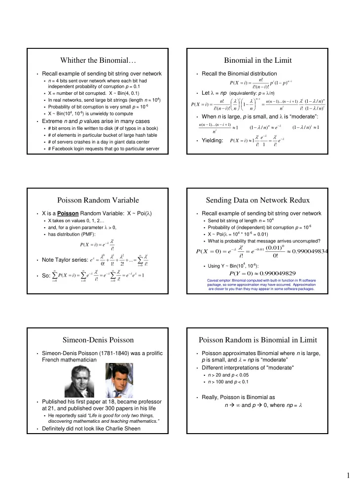
Simeon-Denis Poisson
- Simeon-Denis Poisson (1781-1840) was a prolific
French mathematician
- Published his first paper at 18, became professor
at 21, and published over 300 papers in his life
- He reportedly said “Life is good for only two things,
discovering mathematics and teaching mathematics.”
- Definitely did not look like Charlie Sheen
Poisson Random is Binomial in Limit
- Poisson approximates Binomial where n is large,
p is small, and l = np is “moderate”
- Different interpretations of "moderate"
- n > 20 and p < 0.05
- n > 100 and p < 0.1
- Really, Poisson is Binomial as