1 Discrete Conditional Distributions Operating System Loyalty - - PDF document

1
SMART_READER_LITE
LIVE PREVIEW

1 Discrete Conditional Distributions Operating System Loyalty - - PDF document

Sum of Independent Binomial RVs Sum of Independent Poisson RVs Let X and Y be independent random variables Let X and Y be independent random variables X ~ Poi( l 1 ) and Y ~ Poi( l 2 ) X ~ Bin(n 1 , p) and Y ~ Bin(n 2 , p) X


slide-1
SLIDE 1

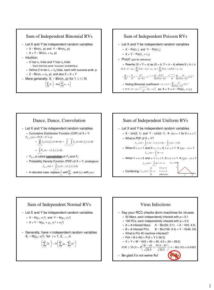
1 Sum of Independent Binomial RVs

  • Let X and Y be independent random variables
  • X ~ Bin(n1, p) and Y ~ Bin(n2, p)
  • X + Y ~ Bin(n1 + n2, p)
  • Intuition:
  • X has n1 trials and Y has n2 trials
  • Each trial has same “success” probability p
  • Define Z to be n1 + n2 trials, each with success prob. p
  • Z ~ Bin(n1 + n2, p), and also Z = X + Y
  • More generally: Xi ~ Bin(ni, p) for 1  i  N

           

 

 

p n X

N i i n i i

, Bin ~

1 1

Sum of Independent Poisson RVs

  • Let X and Y be independent random variables
  • X ~ Poi(l1) and Y ~ Poi(l2)
  • X + Y ~ Poi(l1 + l2)
  • Proof: (just for reference)
  • Rewrite (X + Y = n) as (X = k, Y = n – k) where 0  k  n
  • Noting Binomial coefficient:
  • so, X + Y = n ~ Poi(l1 + l2)

 

 

         

n k n k

k n Y P k X P k n Y k X P n Y X P ) ( ) ( ) , ( ) (

  

           

     

n k k n k n k k n k n k k n k

k n k n n e k n k e k n e k e

2 1 ) ( 2 1 ) ( 2 1

)! ( ! ! ! )! ( ! )! ( !

2 1 2 1 2 1

l l l l l l

l l l l l l

 

n

n e n Y X P

2 1 ) (

! ) (

2 1

l l

l l

   

 

 

  

n k k n k n

k n k n

2 1 2 1

)! ( ! ! ) ( l l l l

Dance, Dance, Convolution

  • Let X and Y be independent random variables
  • Cumulative Distribution Function (CDF) of X + Y:
  • FX+Y is called convolution of FX and FY
  • Probability Density Function (PDF) of X + Y, analogous:
  • In discrete case, replace with , and f(y) with p(y)

) ( ) ( a Y X P a F

Y X

  

  

       

 

y y a x Y X a y x Y X

dy y f dx x f dy dx y f x f ) ( ) ( ) ( ) (

  

 

y Y X

dy y f y a F ) ( ) (

   

 

y Y X Y X

dy y f y a f a f ) ( ) ( ) (

   y

y

Sum of Independent Uniform RVs

  • Let X and Y be independent random variables
  • X ~ Uni(0, 1) and Y ~ Uni(0, 1)  f(a) = 1 for 0  a  1
  • What is PDF of X + Y?
  • When 0  a  1 and 0  y  a, 0  a–y  1  fX(a – y) = 1
  • When 1 < a < 2 and a–1  y  1, 0  a–y  1  fX(a – y) = 1
  • Combining:

 

  

   

1 1

) ( ) ( ) ( ) (

y X y Y X Y X

dy y a f dy y f y a f a f a dy a f

a y Y X

  

 

) ( a dy a f

a y Y X

   

  

2 ) (

1 1

          

  • therwise

2 1 2 1 ) ( a a a a a f

Y X

a 2

1 1

) (a f

Y X 

Sum of Independent Normal RVs

  • Let X and Y be independent random variables
  • X ~ N(m1, s12) and Y ~ N(m2, s22)
  • X + Y ~ N(m1 + m2, s12 + s22)
  • Generally, have n independent random variables

Xi ~ N(mi, si

2) for i = 1, 2, ..., n:

           

  

   n i i n i i n i i

N X

1 2 1 1

, ~ s m

Virus Infections

  • Say your RCC checks dorm machines for viruses
  • 50 Macs, each independently infected with p = 0.1
  • 100 PCs, each independently infected with p = 0.4
  • A = # infected Macs

A ~ Bin(50, 0.1)  X ~ N(5, 4.5)

  • B = # infected PCs

B ~ Bin(100, 0.4)  Y ~ N(40, 24)

  • What is P(≥ 40 machine infected)?
  • P(A + B ≥ 40)  P(X + Y ≥ 39.5)
  • X + Y = W ~ N(5 + 40 = 45, 4.5 + 24 = 28.5)
  • Be glad it’s not swine flu!

8485 . ) 03 . 1 ( 1 5 . 28 45 5 . 39 5 . 28 45 ) 5 . 39 (                W P W P

slide-2
SLIDE 2

2 Discrete Conditional Distributions

  • Recall that for events E and F:
  • Now, have X and Y as discrete random variables
  • Conditional PMF of X given Y (where pY(y) > 0):
  • Conditional CDF of X given Y (where pY(y) > 0):

) ( ) ( ) ( ) | (   F P F P EF P F E P where ) ( ) , ( ) ( ) , ( ) | ( ) | (

, |

y p y x p y Y P y Y x X P y Y x X P y x P

Y Y X Y X

        ) ( ) , ( ) | ( ) | (

|

y Y P y Y a X P y Y a X P y a F

Y X

      

 

 

 

a x Y X Y a x Y X

y x p y p y x p ) | ( ) ( ) , (

| ,

  • Consider person buying 2 computers (over time)
  • X = 1st computer bought is a PC (1 if it is, 0 if it is not)
  • Y = 2nd computer bought is a PC (1 if it is, 0 if it is not)
  • Joint probability mass function (PMF):
  • What is P(Y = 0 | X = 0)?
  • What is P(Y = 1 | X = 0)?
  • What is P(X = 0 | Y = 1)?

Operating System Loyalty

X Y 1 pY(y) 0.2 0.3 0.5 1 0.1 0.4 0.5 pX(x) 0.3 0.7 1.0

3 1 3 . 1 . ) ( ) 1 , ( ) | 1 (

,

    

X Y X

p p X Y P 3 2 3 . 2 . ) ( ) , ( ) | (

,

    

X Y X

p p X Y P 5 1 5 . 1 . ) 1 ( ) 1 , ( ) 1 | (

,

    

Y Y X

p p Y X P

And It Applies to Books Too…

P(Buy Book Y | Bought Book X)

  • Requests received at web server in a day
  • X = # requests from humans/day

X ~ Poi(l1)

  • Y = # requests from bots/day

Y ~ Poi(l2)

  • X and Y are independent  X + Y ~ Poi(l1 + l2)
  • What is P(X = k | X + Y = n)?
  • X | X + Y ~

Web Server Requests Redux

) ( ) ( ) ( ) ( ) , ( ) | ( n Y X P k n Y P k X P n Y X P k n Y k X P n Y X k X P               

n k n k n k n k

k n k n e n k n e k e ) ( )! ( ! ! ) ( ! )! ( !

2 1 2 1 2 1 ) ( 2 1

2 1 2 1

l l l l l l l l

l l l l

        

      k n k

k n

                          

2 1 2 2 1 1

l l l l l l

         

2 1 1

, Bin l l l Y X

Continuous Conditional Distributions

  • Let X and Y be continuous random variables
  • Conditional PDF of X given Y (where fY(y) > 0):
  • Conditional CDF of X given Y (where fY(y) > 0):
  • Note: Even though P(Y = a) = 0, can condition on Y = a
  • Really considering:

) ( ) , ( ) | (

, |

y f y x f y x f

Y Y X Y X

dx y x f y Y a X P y a F

a Y X Y X

) | ( ) | ( ) | (

| |

 

   

dy y f dy dx y x f dx y x f

Y Y X Y X

) ( ) , ( ) | (

, |

 ) | ( ) ( ) , ( dy y Y y dx x X x P dy y Y y P dy y Y y dx x X x P                 

 

     

2 / 2 /

) ( ) ( ) (

2 2

 

 

a a Y

a f dy y f a Y a P

  • X and Y are continuous RVs with PDF:
  • Compute conditional density:

Let’s Do an Example

       

  • therwise

1 ere wh ) 2 ( ) , (

5 12

x,y y x x y x f ) | (

|

y x f

Y X

dx y x f y x f y f y x f y x f

Y X Y X Y Y X Y X

) , ( ) , ( ) ( ) , ( ) | (

1 , , , |

 

 

1 2 3 2 1 1

2 3 5 12 5 12

) 2 ( ) 2 ( ) 2 ( ) 2 ( ) 2 (

y x x x

y x x dx y x x y x x dx y x x y x x

 

            

 

y y x x y x x

y

3 4 ) 2 ( 6 ) 2 (

2 3 2

      

slide-3
SLIDE 3

3 Independence and Conditioning

  • If X and Y are independent discrete RVs:
  • Analogously, for independent continuous RVs:

) ( ) ( ) ( ) ( ) ( ) , ( ) | ( x X P y Y P y Y P x X P y Y P y Y x X P y Y x X P             ) ( ) ( ) ( ) ( ) ( ) , ( ) | (

, |

x f y f y f x f y f y x f y x f

X Y Y X Y Y X Y X

   ) ( ) ( ) ( ) ( ) ( ) , ( ) | (

, |

x p y p y p x p y p y x p y x p

X Y Y X Y Y X Y X

  

Conditional Independence Revisited

  • n discrete random variables X1, X2, …, Xn are

called conditionally independent given Y if:

  • Analogously, for continuous random variables:
  • Note: can turn products into sums using logs:

y a a a y Y a X P y Y a X a X a X P

n i i n i n n

, ,..., , all for ) | ( ) | ,..., , (

2 1 1 2 2 1 1

      

y x x x y Y x X P y Y x X x X x X P

n i i n i n n

, ,..., , all for ) | ( ) | ,..., , (

2 1 1 2 2 1 1

      

K y Y x X P y Y x X P

i i n i i i

     

 

  n 1 i 1

) | ( ln ) | ( ln

K n i i i

e y Y x X P ) | (

1

  

Mixing Discrete and Continuous

  • Let X be a continuous random variable
  • Let N be a discrete random variable
  • Conditional PDF of X given N:
  • Conditional PMF of N given X:
  • If X and N are independent, then:

) ( ) ( ) | ( ) | (

| |

n p x f x n p n x f

N X X N N X

 ) ( ) ( ) | ( ) | (

| |

x f n p n x f x n p

X N N X X N

) ( ) | (

|

x f n x f

X N X

 ) ( ) | (

|

n p x n p

N X N

Beta Random Variable

  • X is a Beta Random Variable: X ~ Beta(a, b)
  • Probability Density Function (PDF):

where

  • Symmetric when a = b

      

 

  • therwise

1 ) (

1 1

) 1 ( ) , ( 1

x x f

b a

x x b a B

 

 

1 1 1

) 1 ( ) , ( dx x x b a B

b a

b a a X E   ] [ ) 1 ( ) ( ) (

2

    b a b a ab X Var

  • Flip a coin (n + m) times, comes up with n heads
  • We don’t know probability X that coin comes up heads
  • All we know is that: X ~ Uni(0, 1)
  • What is density of X given n heads in n + m flips?
  • Let N = number of heads
  • Given X = x, coin flips independent: N | X ~ Bin(n + m, x)
  • Compute conditional density of X given N = n

Flipping Coin With Unknown Probability

) ( ) 1 ( ) ( ) ( ) | ( ) | (

|

n N P x x n N P x f x X n N P n x f

m n X N X

n m n

            

    

1

) 1 ( ) 1 ( 1 dx x x c x x c

m n m n

where

1

  • Flip a coin (n + m) times, comes up with n heads
  • Conditional density of X given N = n
  • Note:
  • Recall Beta distribution:
  • Hey, that looks more familiar now...
  • X | (N = n, n + m trials) ~ Beta(n + 1, m + 1)

Dude, Where’s My Beta?!

    

1 |

) 1 ( ) 1 ( 1 ) | ( dx x x c x x c n x f

m n m n N X

where

       

 

  • therwise

1 ) (

1 1

) 1 ( ) , ( 1

x x f

b a

x x b a B

 

 

1 1 1

) 1 ( ) , ( dx x x b a B

b a

  • therwise

so ) | ( , 1

|

   n x f x

N X

slide-4
SLIDE 4

4

  • X | (N = n, m + n trials) ~ Beta(n + 1, m + 1)
  • X ~ Uni(0, 1)
  • Check this out, boss:
  • Beta(1, 1) = Uni(0, 1)
  • So, X ~ Beta(1, 1)
  • “Prior” distribution of X (before seeing any flips) is Beta
  • “Posterior” distribution of X (after seeing flips) is Beta
  • Beta is a conjugate distribution for Beta
  • Prior and posterior parametric forms are the same!
  • Beta is also conjugate for Bernoulli and Binomial
  • Practically, conjugate means easy update:
  • Add number of “heads” and “tails” seen to Beta parameters

Understanding Beta

1 where 1 1 1 1

1

     x dx

1 1

) 1 ( ) , ( 1 ) 1 ( ) , ( 1 ) ( x x b a B x x b a B x f

b a

   

 

  • Can set X ~ Beta(a, b) as prior to reflect how

biased you think coin is apriori

  • This is a subjective probability!
  • Then observe n + m trials,

where n of trials are heads

  • Update to get posterior probability
  • X | (n heads in n + m trials) ~ Beta(a + n, b + m)
  • Sometimes call a and b the “equivalent sample size”
  • Prior probability for X based on seeing (a + b – 2)

“imaginary” trials, where (a – 1) of them were heads.

  • Beta(1, 1) ~ Uni(0, 1)  we haven’t seen any

“imaginary trials”, so apriori know nothing about coin

Further Understanding Beta