kinkyreg instrument free inference for linear regression
play

kinkyreg: Instrument-free inference for linear regression models - PowerPoint PPT Presentation

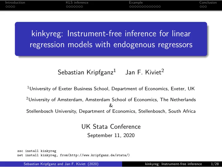
Introduction KLS inference Example Conclusion kinkyreg: Instrument-free inference for linear regression models with endogenous regressors Sebastian Kripfganz 1 Jan F. Kiviet 2 1 University of Exeter Business School, Department of Economics,


  1. Introduction KLS inference Example Conclusion kinkyreg: Instrument-free inference for linear regression models with endogenous regressors Sebastian Kripfganz 1 Jan F. Kiviet 2 1 University of Exeter Business School, Department of Economics, Exeter, UK 2 University of Amsterdam, Amsterdam School of Economics, The Netherlands & Stellenbosch University, Department of Economics, Stellenbosch, South Africa UK Stata Conference September 11, 2020 ssc install kinkyreg net install kinkyreg, from(http://www.kripfganz.de/stata/) Sebastian Kripfganz and Jan F. Kiviet (2020) kinkyreg: Instrument-free inference 1/28

  2. Introduction KLS inference Example Conclusion Instrument-based versus instrument-free inference Instrumental variables dominate the empirical literature on causal inference in linear regression models with endogenous regressors. For valid inference under conventional asymptotics, instruments must be relevant and exogenous. Weak instruments can lead to severe coefficient biases, poor approximations of the finite-sample distributions, and large size distortions of statistical tests. Robust statistical inference in the presence of weak instruments is possible but usually leads to wide and often not very informative confidence intervals. Literature overview: Stock, Wright, and Yogo (2002), Andrews and Stock (2007), and Andrews, Stock, and Sun (2019). Sebastian Kripfganz and Jan F. Kiviet (2020) kinkyreg: Instrument-free inference 2/28

  3. Introduction KLS inference Example Conclusion Instrument-based versus instrument-free inference Community-contributed Stata commands for weak-instruments tests and weak-instruments robust inference: ivreg2 (Baum, Schaffer, and Stillman, 2003, 2007), condivreg (Moreira and Poi, 2003; Mikusheva and Poi, 2006), rivtest (Finlay and Magnusson, 2009), weakivtest (Pflueger and Wang, 2015), twostepweakiv (Sun, 2018). The same features that make an instrument relevant can also be a source of a violation of the exogeneity condition (Hall, Rudebusch, and Wilcox, 1996). Sebastian Kripfganz and Jan F. Kiviet (2020) kinkyreg: Instrument-free inference 3/28

  4. Introduction KLS inference Example Conclusion Instrument-based versus instrument-free inference Exogeneity of an instrument necessitates that it is validly excluded from the structural model. In just-identified models, this exclusion restriction is untestable in the standard instrumental variables framework. Even in overidentified models, routinely used overidentification tests rely on the maintained assumption that at least as many instruments are validly excluded as there are endogenous regressors (Parente and Santos Silva, 2012). Alternative assumptions can be imposed to enable testing of the exclusion restrictions. Sebastian Kripfganz and Jan F. Kiviet (2020) kinkyreg: Instrument-free inference 4/28

  5. Introduction KLS inference Example Conclusion Instrument-based versus instrument-free inference We present the new kinkyreg Stata command for kinky least squares (KLS) estimation (Kiviet, 2020a,b) that does not rely on instrumental variables: KLS analytically corrects the bias of OLS for all values of the endogeneity correlations on a specified grid. Set identification is achieved by confining the admissible degree of regressor endogeneity within plausible bounds. For a reasonably narrow range of endogeneity correlations, KLS confidence intervals are often narrower than those from 2SLS, in particular if instruments are weak, or other instrument-based methods (e.g. the approach of “plausibly exogenous” instruments by Conley, Hansen, and Rossi, 2012). Exclusion restrictions are testable within the KLS framework. Sebastian Kripfganz and Jan F. Kiviet (2020) kinkyreg: Instrument-free inference 5/28

  6. Introduction KLS inference Example Conclusion Linear regression model Linear regression model with an endogenous regressor x 1 i and exogenous regressors x 2 i (all variables in deviations from their mean): y i = β 1 x 1 i + x ′ 2 i β 2 + ε i , with ε i ∼ (0 , σ 2 ε ) and � � �� � � �� σ 2 x 1 i 0 σ ′ 1 12 ∼ , . x 2 i 0 σ 12 Σ 2 The model can be generalized for multiple endogenous regressors (Kiviet, 2020a,b). OLS is inconsistent because E [ x 1 i ε i ] = ρ σ 1 σ ε � = 0 for nonzero endogeneity correlations Corr ( x 1 i , ε i ) = ρ � = 0. Sebastian Kripfganz and Jan F. Kiviet (2020) kinkyreg: Instrument-free inference 6/28

  7. Introduction KLS inference Example Conclusion Kinky least squares estimation While 2SLS uses orthogonality conditions E [ z i ε i ] = 0 , KLS utilizes the non-orthogonality condition E [ x 1 i ε i ] = ρ σ 1 σ ε (in addition to the orthogonality conditions for the exogenous regressors x 2 i ). For a given correlation ρ , σ ε can be consistently estimated as the square root of − 1   σ 2 ˆ σ 2 σ 2  1 − ρ 2 1 ˆ ε ( ρ ) = ˆ , ε, OLS  − 1 12 ˆ σ 2 σ ′ ˆ 1 − ˆ Σ 2 ˆ σ 12 σ 2 ε, OLS = N − 1 � N ε 2 where ˆ i =1 ˆ i , OLS , with OLS residuals ˆ ε i , OLS . σ 12 , and ˆ σ 2 The variance estimates ˆ 1 , ˆ Σ 2 are readily obtained from the data. Sebastian Kripfganz and Jan F. Kiviet (2020) kinkyreg: Instrument-free inference 7/28

  8. Introduction KLS inference Example Conclusion Kinky least squares estimation The KLS estimator corrects the inconsistency of the OLS estimator: � ˆ � ˆ � � � � 1 ρ ˆ σ 1 ˆ σ ε ( ρ ) β 1 ( ρ ) β 1 , OLS = − . − 1 ˆ ˆ − ˆ − 1 β 2 ( ρ ) β 2 , OLS 12 ˆ Σ 2 ˆ σ 12 σ 2 ˆ 1 − ˆ σ ′ 2 ˆ Σ σ 12 Kiviet (2020a,b) derives an analytical expression for the variance-covariance matrix of the KLS estimator, σ 2 ε V ( ρ, κ x , κ ε ), as a function of the kurtosis of the regressors, κ x , and the kurtosis of the error term, κ ε . Estimates of κ x can be obtained from the data, and κ ε ( ρ ) = N − 1 � N σ ε ( ρ )] 4 , with KLS residuals ˆ ˆ i =1 [ˆ ε i ( ρ ) / ˆ ε i ( ρ ). For a tractable expression of V ( ρ, κ x , κ ε ), Kiviet (2020a,b) assumes an identical kurtosis κ x for all regressors. By choosing κ x as the maximum of the individual kurtosis estimates, we ˆ obtain (asymptotically) conservative confidence intervals. Sebastian Kripfganz and Jan F. Kiviet (2020) kinkyreg: Instrument-free inference 8/28

  9. Introduction KLS inference Example Conclusion Kinky least squares estimation The endogeneity correlation ρ is unknown but assumed to lie in the interval ρ ∈ [ r l , r u ]. The KLS estimator ˆ β ( r ) is computed for a range of values r ∈ [ r l , r u ], subject to the feasibility bounds � − 1 12 ˆ � σ ′ � 1 − ˆ Σ 2 ˆ σ 12 � | r | < ≤ 1 . σ 2 ˆ 1 For a significance level α , the union of KLS confidence intervals over the range r ∈ [ r l , r u ] has asymptotic coverage of at least 1 − α . Sebastian Kripfganz and Jan F. Kiviet (2020) kinkyreg: Instrument-free inference 9/28

  10. Introduction KLS inference Example Conclusion kinkyreg command syntax kinkyreg depvar [ varlist1 ] ( varlist2 [= varlist iv ]) [ if ] [ in ], [ options ] Basic command syntax similar to ivregress , but instrumental variables are optional: Main options (see the Stata help file for a full list): endogeneity ( numlist ) to specify values for the fixed endogeneity correlations of the endogenous regressors varlist2 , range (# 1 # 2 ) to specify the admissible endogeneity range, stepsize (#) to specify the step size, small to report small-sample statistics, inference ( varlist ) to specify the variables for graphical KLS inference, lincom (#: exp ) to specify linear combinations for graphical KLS inference, options to modify the appearance of the KLS graphs. Sebastian Kripfganz and Jan F. Kiviet (2020) kinkyreg: Instrument-free inference 10/28

  11. Introduction KLS inference Example Conclusion Specification tests Linear hypotheses tests (Wald/F tests) for H 0 : R β = c : � − 1 � � ′ � � � ˆ R ˆ σ 2 R ˆ W ( r ) = β ( r ) − c ˆ ε ( r ) V ( r , ˆ κ x , ˆ κ ε ( r )) β ( r ) − c , with postestimation command estat test . Exclusion restriction tests for instrumental variables (or other variables) x 3 , i.e. H 0 : β 3 = 0 in the auxiliary model y i = β 1 x 1 i + x ′ 2 i β 2 + x ′ 3 i β 3 + ε i , with postestimation command estat exclusion . Sebastian Kripfganz and Jan F. Kiviet (2020) kinkyreg: Instrument-free inference 11/28

  12. Introduction KLS inference Example Conclusion Specification tests Ramsey’s RESET test, i.e. an exclusion restrictions test for higher-order polynomials of the fitted values or right-hand side variables, with postestimation command estat reset . Breusch-Pagan heteroskedasticity tests, with postestimation command estat hettest . Durbin’s “alternative test” for serial correlation, with postestimation command estat durbinalt . All specification tests are computed over the same range of endogeneity correlations r ∈ [ r l , r u ]. Sebastian Kripfganz and Jan F. Kiviet (2020) kinkyreg: Instrument-free inference 12/28

Download Presentation
Download Policy: The content available on the website is offered to you 'AS IS' for your personal information and use only. It cannot be commercialized, licensed, or distributed on other websites without prior consent from the author. To download a presentation, simply click this link. If you encounter any difficulties during the download process, it's possible that the publisher has removed the file from their server.

Recommend


More recommend