1 Dont Make Me Get Non -Linear! A Grounding Example: Linear - - PDF document

1
SMART_READER_LITE
LIVE PREVIEW

1 Dont Make Me Get Non -Linear! A Grounding Example: Linear - - PDF document

What is Machine Learning? A (Very Short) List of Applications Many different forms of Machine Learning Machine learning widely used in many contexts We focus on the problem of prediction Stock price prediction o Using economic


slide-1
SLIDE 1

1 What is Machine Learning?

  • Many different forms of “Machine Learning”
  • We focus on the problem of prediction
  • Want to make a prediction based on observations
  • Vector X of m observed variables: <X1, X2, …, Xm>
  • X1, X2, …, Xm are called “input features/variables”
  • Also called “independent variables,” but this can be misleading!
  • X1, X2, …, Xm need not be (and usually are not) independent
  • Based on observed X, want to predict unseen variable Y
  • Y called “output feature/variable” (or the “dependent variable”)
  • Seek to “learn” a function g(X) to predict Y:
  • When Y is discrete, prediction of Y is called “classification”
  • When Y is continuous, prediction of Y is called “regression”

) ( ˆ X g Y 

A (Very Short) List of Applications

  • Machine learning widely used in many contexts
  • Stock price prediction
  • Using economic indicators, predict if stock with go up/down
  • Computational biology and medical diagnosis
  • Predicting gene expression based on DNA
  • Determine likelihood for cancer using clinical/demographic data
  • Predict people likely to purchase product or click on ad
  • “Based on past purchases, you might want to buy…”
  • Credit card fraud and telephone fraud detection
  • Based on past purchases/phone calls is a new one fraudulent?
  • Saves companies billions(!) of dollars annually
  • Spam E-mail detection (gmail, hotmail, many others)

What is Bayes Doing in My Mail Server?

  • This is spam:

Who was crazy enough to think of that?

Let’s get Bayesian on your spam:

Content analysis details: (49.5 hits, 7.0 required) 0.9 RCVD_IN_PBL RBL: Received via a relay in Spamhaus PBL [93.40.189.29 listed in zen.spamhaus.org] 1.5 URIBL_WS_SURBL Contains an URL listed in the WS SURBL blocklist [URIs: recragas.cn] 5.0 URIBL_JP_SURBL Contains an URL listed in the JP SURBL blocklist [URIs: recragas.cn] 5.0 URIBL_OB_SURBL Contains an URL listed in the OB SURBL blocklist [URIs: recragas.cn] 5.0 URIBL_SC_SURBL Contains an URL listed in the SC SURBL blocklist [URIs: recragas.cn] 2.0 URIBL_BLACK Contains an URL listed in the URIBL blacklist [URIs: recragas.cn] 8.0 BAYES_99 BODY: Bayesian spam probability is 99 to 100% [score: 1.0000]

Spam, Spam… Go Away!

  • The constant battle with spam

Source: http://www.google.com/mail/help/fightspam/spamexplained.html “And machine-learning algorithms developed to merge and rank large sets of Google search results allow us to combine hundreds of factors to classify spam.”

Training a Learning Machine

  • We consider statistical learning paradigm here
  • We are given set of N “training” instances
  • Each training instance is pair: (<x1, x2, …, xm>, y)
  • Training instances are previously observed data
  • Gives the output value y associated with each observed vector
  • f input values <x1, x2, …, xm>
  • Learning: use training data to specify g(X)
  • Generally, first select a parametric form for g(X)
  • Then, estimate parameters of model g(X) using training data
  • For regression, usually want g(X) that minimizes E[(Y – g(X))2]
  • Mean squared error (MSE) “loss” function. (Others exist.)
  • For classification, generally best choice of

) | ( ˆ max arg ) ( X X Y P g

y

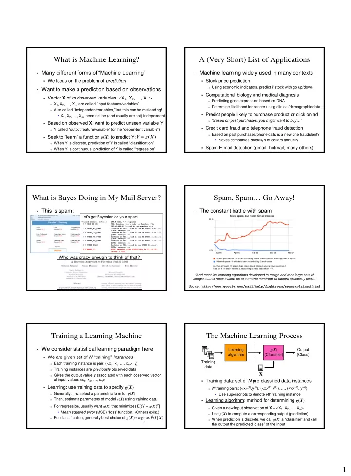
The Machine Learning Process

  • Training data: set of N pre-classified data instances
  • N training pairs: (<x>(1),y(1)), (<x>(2),y(2)), …, (<x>(N), y(N))
  • Use superscripts to denote i-th training instance
  • Learning algorithm: method for determining g(X)
  • Given a new input observation of X = <X1, X2, …, Xm>
  • Use g(X) to compute a corresponding output (prediction)
  • When prediction is discrete, we call g(X) a “classifier” and call

the output the predicted “class” of the input Output (Class) Training data Learning algorithm g(X) (Classifier)

X

slide-2
SLIDE 2

2 A Grounding Example: Linear Regression

  • Predict real value Y based on observing variable X
  • Assume model is linear:
  • Training data
  • Each vector X has one observed variable: <X1> (just call it X)
  • Y is continuous output variable
  • Given N training pairs: (<x>(1),y(1)), (<x>(2),y(2)), …, (<x>(N), y(N))
  • Use superscripts to denote i-th training instance
  • Determine a and b minimizing E[(Y – g(X))2]
  • First, minimize objective function:

b aX g Y    ) ( ˆ X ] ) [( ] )) ( [( ] )) ( [(

2 2 2

b aX Y E b aX Y E X g Y E       

Don’t Make Me Get Non-Linear!

  • Minimize objective function
  • Compute derivatives w.r.t. a and b
  • Set derivatives to 0 and solve simultaneous equations:
  • Substitution yields:
  • Estimate parameters based on observed training data:

] ) [(

2

b aX Y E  

] [ 2 ] [ 2 ] [ 2 )] ( 2 [ ] ) [(

2 2

X bE X aE XY E b aX Y X E b aX Y E a             b X aE Y E b aX Y E b aX Y E b 2 ] [ 2 ] [ 2 )] ( 2 [ ] ) [(

2

           

x y

Y X X Var Y X Cov X E X E Y E X E XY E a    ) , ( ) ( ) , ( ]) [ ( ] [ ] [ ] [ ] [

2 2

    

x x y y

Y X X aE Y E b      ) , ( ] [ ] [    

y x x y X

Y X Y         ) ( ) , ( Y X x Y X x X g Y

x y

     ) ( ˆ ˆ ) , ( ˆ ) ( ˆ   

A Simple Classification Example

  • Predict Y based on observing variable X
  • X has discrete value from {1, 2, 3, 4}
  • X denotes temperature range today: <50, 50-60, 60-70, >70
  • Y has discrete value from {rain, sun}
  • Y denotes general weather outlook tomorrow
  • Given training data, estimate joint PMF:
  • Note Bayes rule:
  • For new X, predict
  • Note px(x) is not affected by choice of y, yielding:

) ( ) ( ) | ( ) ( ) , ( ) | (

, ,

x p y p y x p x p y x p X Y P

X Y Y X X Y X

 

) , ( ˆ

,

y x p

Y X

) | ( ˆ max arg ) ( ˆ X Y P g Y

y

  X ) ( ˆ ) | ( ˆ max arg ) , ( ˆ max arg ) | ( ˆ max arg ) ( ˆ Y P Y X P Y X P X Y P g Y

y y y

    X

Estimating the Joint PMF

  • Given training data, compute joint PMF: pX,Y(x, y)
  • MLE: count number of times each pair (x, y) appears
  • MAP using Laplace prior: add 1 to all the MLE counts
  • Normalize to get true distribution (sums to 1)
  • Observed 50 data points:

X Y 1 2 3 4 pY(y) rain 0.10 0.06 0.04 0.00 0.20 sun 0.06 0.14 0.20 0.40 0.80 pX(x) 0.16 0.20 0.24 0.40 1.00 X Y 1 2 3 4 rain 5 3 2 sun 3 7 10 20 X Y 1 2 3 4 pY(y) rain 0.103 0.069 0.052 0.017 0.241 sun 0.069 0.138 0.190 0.362 0.759 pX(x) 0.172 0.207 0.242 0.379 1.00 MLE estimate Laplace (MAP) estimate points data # total cell in count ˆ 

MLE

p cells # total points data # total 1 cell in count ˆ   

Laplace

p

Classify New Observation

  • Say today’s temperature is 75, so X = 4
  • Recall X temperature ranges: <50, 50-60, 60-70, >70
  • Prediction for Y (weather outlook tomorrow)
  • What if we asked what is probability of rain tomorrow?
  • MLE: absolutely, positively no chance of rain!
  • Laplace estimate: very small (~2%) chance  “never say never”

) ( ˆ ) | ( ˆ max arg ) , ( ˆ max arg ˆ Y P Y X P Y X P Y

y y

 

X Y 1 2 3 4 pY(y) rain 0.10 0.06 0.04 0.00 0.20 sun 0.06 0.14 0.20 0.40 0.80 pX(x) 0.16 0.20 0.24 0.40 1.00

MLE estimate

X Y 1 2 3 4 pY(y) rain 0.103 0.069 0.052 0.017 0.241 sun 0.069 0.138 0.190 0.362 0.759 pX(x) 0.172 0.207 0.242 0.379 1.00

Laplace (MAP) estimate

Classification with Multiple Observables

  • Say, we have m input values X = <X1, X2, …, Xm>
  • Note that variables X1, X2, …, Xm can de dependent!
  • In theory, could predict Y as before, using
  • Why won’t this necessarily work?
  • Need to estimate P(X1, X2, …, Xm | Y)
  • Fine if m is small, but what if m = 10 or 100 or 10,000?
  • Note: size of PMF table is exponential in m (e.g. O(2m))
  • Need ridiculous amount of data for good probability estimates!
  • Likely to have many 0’s in table (bad times)
  • Need to consider a simpler model

) ( ˆ ) | ( ˆ max arg ) , ( ˆ max arg ˆ Y P Y P Y P Y

y y

X X  

slide-3
SLIDE 3

3 Naive Bayesian Classifier

  • Say, we have m input values X = <X1, X2, …, Xm>
  • Assume variables X1, X2, …, Xm are conditionally

independent given Y

  • Really don’t believe X1, X2, …, Xm are conditionally independent
  • Just an approximation we make to be able to make predictions
  • This is called the “Naive Bayes” assumption, hence the name
  • Predict Y using
  • But, we now have:

by conditional independence

  • Note: computation of PMF table is linear in m : O(m)
  • Don’t need much data to get good probability estimates

 

m i i m

Y X P Y X X X P Y P

1 2 1

) | ( ) | ,... , ( ) | (X ) ( ) | ( max arg ) , ( max arg ˆ Y P Y P Y P Y

y y

X X  

Email Classification

  • Want to predict is an email is spam or not
  • Start with the input data
  • Consider a lexicon of m words (Note: in English m  100,000)
  • Define m indicator variables X = <X1, X2, …, Xm>
  • Each variable Xi denotes if word i appeared in a document or not
  • Note: m is huge, so make “Naive Bayes” assumption
  • Define output classes Y to be: {spam, non-spam}
  • Given training set of N previous emails
  • For each email message, we have a training instance:

X = <X1, X2, …, Xm> noting for each word, if it appeared in email

  • Each email message is also marked as spam or not (value of Y)

Training the Classifier

  • Given N training pairs:

(<x>(1),y(1)), (<x>(2),y(2)), …, (<x>(N), y(N))

  • Learning
  • Estimate probabilities P(Y) and each P(Xi | Y) for all i
  • Many words are likely to not appear at all in given set of email
  • Use Laplace estimate:
  • Classification
  • For a new email, generate X = <X1, X2, …, Xm>
  • Classify as spam or not using:
  • Employ Naive Bayes assumption:

) ( ˆ ) | ( ˆ max arg ˆ Y P Y P Y

y

X 

m i i Y

X P Y P

1

) | ( ˆ ) | ( ˆ X

2 emails spam # total 1 with word emails spam # ) | ( ˆ     i spam Y X p

Laplace i

How Does This Do?

  • After training, can test with another set of data
  • “Testing” set also has known values for Y, so we can

see how often we were right/wrong in predictions for Y

  • Spam data
  • Email data set: 1789 emails (1578 spam, 211 non-spam)
  • First, 1538 email messages (by time) used for training
  • Next 251 messages used to test learned classifier
  • Criteria:
  • Precision = # correctly predicted class Y/ # predicted class Y
  • Recall = # correctly predicted class Y / # real class Y messages

Spam Non-spam Precision Recall Precision Recall Words only 97.1% 94.3% 87.7% 93.4% Words + add’l features 100% 98.3% 96.2% 100%

A Little Text Analysis of the Governator

  • Arnold Schwarzenegger’s actual veto letter:

Coincidence, You Ask?

  • San Francisco Chronicle, Oct. 28, 2009:

“Schwarzenegger's press secretary, Aaron McLear, insisted Tuesday it was simply a „weird coincidence‟."

  • Steve Piantadosi (grad student at MIT) blog post,
  • Oct. 28, 2009:
  • “…assume that each word starting a line is chosen

independently…”

  • “…[compute] the (token) frequency with which each

letter appears at the start of a word…”

  • Multiply probabilities for letter starting each word of

each line to get final answer: “one in 1 trillion”

  • 50,000 times less likely than winning CA lottery