[PPT] - Component Analysis for PR & HS Component Analysis for PR & PowerPoint Presentation

SLIDE 1

1

PAVIS school on CV and PR

7

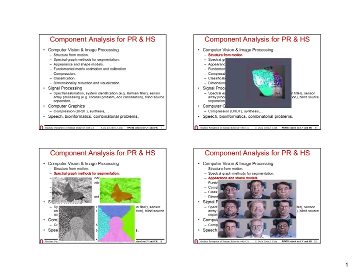
Component Analysis for PR & HS

Computer Vision & Image Processing

– Structure from motion. – Spectral graph methods for segmentation. – Appearance and shape models. – Fundamental matrix estimation and calibration. – Compression. – Classification. – Dimensionality reduction and visualization.

Signal Processing

– Spectral estimation, system identification (e.g. Kalman filter), sensor array processing (e.g. cocktail problem, eco cancellation), blind source separation, -

Computer Graphics

– Compression (BRDF), synthesis,-

Speech, bioinformatics, combinatorial problems.
PAVIS school on CV and PR

8

Computer Vision & Image Processing

– Structure from motion. – Spectral graph methods for segmentation. – Appearance and shape models. – Fundamental matrix estimation and calibration. – Compression. – Classification. – Dimensionality reduction and visualization.

Signal Processing

– Spectral estimation, system identification (e.g. Kalman filter), sensor array processing (e.g. cocktail problem, eco cancellation), blind source separation, -

Computer Graphics

– Compression (BRDF), synthesis,-

Speech, bioinformatics, combinatorial problems.

Structure from motion

Component Analysis for PR & HS

PAVIS school on CV and PR

9

Computer Vision & Image Processing

– Structure from motion. – Spectral graph methods for segmentation. – Appearance and shape models. – Fundamental matrix estimation and calibration. – Compression. – Classification. – Dimensionality reduction and visualization.

Signal Processing

– Spectral estimation, system identification (e.g. Kalman filter), sensor array processing (e.g. cocktail problem, eco cancellation), blind source separation, -

Computer Graphics

– Compression (BRDF), synthesis,-

Speech, bioinformatics, combinatorial problems.

Spectral graph methods for segmentation.

Component Analysis for PR & HS

PAVIS school on CV and PR 10
Computer Vision & Image Processing

– Structure from motion. – Spectral graph methods for segmentation. – Appearance and shape models. – Fundamental matrix estimation and calibration. – Compression. – Classification. – Dimensionality reduction and visualization.

Signal Processing

– Spectral estimation, system identification (e.g. Kalman filter), sensor array processing (e.g. cocktail problem, eco cancellation), blind source separation, -

Computer Graphics

– Compression (BRDF), synthesis,-

Speech, bioinformatics, combinatorial problems.

Appearance and shape models

Component Analysis for PR & HS

SLIDE 2

2

PAVIS school on CV and PR 11
Computer Vision & Image Processing

– Structure from motion. – Spectral graph methods for segmentation. – Appearance and shape models. – Fundamental matrix estimation and calibration. – Compression. – Classification. – Dimensionality reduction and visualization.

Signal Processing

– Spectral estimation, system identification (e.g. Kalman filter), sensor array processing (e.g. cocktail problem, eco cancellation), blind source separation, -

Computer Graphics

– Compression (BRDF), synthesis,-

Speech, bioinformatics, combinatorial problems.

Dimensionality reduction and visualization

Component Analysis for PR & HS

PAVIS school on CV and PR 12
Computer Vision & Image Processing

– Structure from motion. – Spectral graph methods for segmentation. – Appearance and shape models. – Fundamental matrix estimation and calibration. – Compression. – Classification. – Dimensionality reduction and visualization.

Signal Processing

– Spectral estimation, system identification (e.g. Kalman filter), sensor array processing (e.g. cocktail problem, eco cancellation), blind source separation, -

Computer Graphics

– Compression (BRDF), synthesis,-

Speech, bioinformatics, combinatorial problems.

cocktail problem

Component Analysis for PR & HS

PAVIS school on CV and PR 13

Independent Component Analysis (ICA)

Sound Source 1 Sound Source 2 Mixture 1 Mixture 2 Output 1 Output 2 I C A Sound Source 3 Mixture 3 Output 3

PAVIS school on CV and PR 14

Why CA for PR & HS?

Learn from high dimensional data and few samples.

– Useful for dimensionality reduction specially when functions are smooth.

features samples

Efficient methods O( d n< <n2 )

(Everitt,1984)

Easy to formulate, to solve and to extend

– Non@linearities (Kernel methods) (Scholkopf & Smola,2002; Shawe@Taylor &

Cristianini,2004)

– Probabilistic (latent variable models) – Multi@factorial (tensors) (Paatero & Tapper, 1994 ;O’Leary & Peleg,1983;

Vasilescu & Terzopoulos,2002; Vasilescu & Terzopoulos,2003)

– Exponential family PCA (Gordon,2002; Collins et al. 01)

Natural geometric interpretation

SLIDE 3

3

PAVIS school on CV and PR 15

Are CA methods popular/useful/used?

Still work to do

– Results 1 10 of about 83,000 for “Spanish crisis" – Results 1 @ 10 of about 287,000,000 for "Britney Spears"

About 28% of CVPR@07 papers use CA.
Google:

– Results 1 @ 10 of about 1,870,000 for "principal component analysis". – Results 1 @ 10 of about 506,000 for "independent component analysis" – Results 1 @ 10 of about 273,000 for "linear discriminant analysis" – Results 1 @ 10 of about 46,100 for "negative matrix factorization" – Results 1 @ 10 of about 491,000 for "kernel methods"

PAVIS school on CV and PR 16

Outline

Introduction (15 min)
Generative models (40 min)

– (PCA, k@means, spectral clustering, NMF, ICA, MDS)

Discriminative models (40 min)

– (LDA, SVM, OCA, CCA)

Standard extensions of linear models (30 min)

–

(Kernel methods, Latent variable models, Tensor factorization )

Unified view (20 min)

Generative models (40 min)

(PCA, k@means, spectral clustering, NMF, ICA, MDS)

PAVIS school on CV and PR 17

Generative models

Principal Component Analysis/Singular Value

Decomposition

Non@Negative Matrix Factorization
Independent Component Analysis
K@means and spectral clustering
Multi@dimensional Scaling

BC D ≈

PAVIS school on CV and PR 18

Principal Component Analysis (PCA)

PCA finds the directions of maximum variation of the data
PCA decorrelates the original variables

(Pearson, 1901; Hotelling, 1933;Mardia et al., 1979; Jolliffe, 1986; Diamantaras, 1996)

+*+=+ @*@ =+

      = Σ

!
!
"
#
$


     = Σ #

#
#
$

+*+=+ @*@ =+ +*@=@ +*@=@

SLIDE 4

4

PAVIS school on CV and PR 19

PCA

+

+ + + ≈

$

#

b

b b $ #

[ ]

1

BC d d d D + ≈ =

$

#

#

× × × ×

ℜ ∈ ℜ ∈ ℜ ∈ ℜ ∈

C

B D

Assuming zero mean data, the basis B that preserve the

maximum variation of the signal is given by the eigenvectors

f DDT.

B Λ B DD =

d

d=pixels

PAVIS school on CV and PR 20

Snap@shot method & SVD

If d>>n (e.g., images 100*100 vs. 300 samples) no DDT.
DDT and DTD have the same eigenvalues (energy) and

related eigenvectors (by D).

B is a linear combination of the data!
[α,L]=eig(DTD) B=D α(diag(diag(L))) @0.5

Λ Dα D Dα DD D BΛ B DD

=

=

SVD PCA

Σ

I V V I U U V Σ U V UΣ D

T T

= = ℜ ∈ ℜ ∈ ℜ ∈ =

× × ×

SVD factorizes the data matrix D as:

Λ = = ℜ ∈ ℜ ∈ =

× × T T

CC I B B C B BC D

U

UΛ DD =

V

VΛ D D =

(Beltrami, 1873; Schmidt, 1907; Golub & Loan, 1989) (Sirovich, 1987)

Dα B =

PAVIS school on CV and PR 21

Error function for PCA

(Eckardt & Young, 1936; Gabriel & Zamir, 1979; Baldi & Hornik, 1989; Shum et al., 1995; De la Torre & Black, 2003a)

Not unique solution:
×

−

ℜ ∈ = R BC C BRR

#

(De la Torre 2012)

BC

D Bc d C B, − = − = ∑

=# $ $ #

% &

PCA minimizes the following function:

(Baldi & Hornik, 1989)

PAVIS school on CV and PR 22

PCA/SVD in Computer Vision

PCA/SVD has been applied to:

– Recognition (eigenfaces:Turk & Pentland, 1991; Sirovich & Kirby, 1987; Leonardis &

Bischof, 2000; Gong et al., 2000; McKenna et al., 1997a)

– Parameterized motion models (Yacoob & Black, 1999; Black et al., 2000; Black,

1999; Black & Jepson, 1998)

– Appearance/shape models (Cootes & Taylor, 2001; Cootes et al., 1998; Pentland

et al., 1994; Jones & Poggio, 1998; Casia & Sclaroff, 1999; Black & Jepson, 1998; Blanz & Vetter, 1999; Cootes et al., 1995; McKenna et al., 1997; de la Torre et al., 1998b; de la Torre et al., 1998b)

– Dynamic appearance models (Soatto et al., 2001; Rao, 1997; Orriols & Binefa,

2001; Gong et al., 2000)

– Structure from Motion (Tomasi & Kanade, 1992; Bregler et al., 2000; Sturm &

Triggs, 1996; Brand, 2001)

– Illumination based reconstruction (Hayakawa, 1994) – Visual servoing (Murase & Nayar, 1995; Murase & Nayar, 1994) – Visual correspondence (Zhang et al., 1995; Jones & Malik, 1992) – Camera motion estimation (Hartley, 1992; Hartley & Zisserman, 2000) – Image watermarking (Liu & Tan, 2000) – Signal processing (Moonen & de Moor, 1995) – Neural approaches (Oja, 1982; Sanger, 1989; Xu, 1993) – Bilinear models (Tenenbaum & Freeman, 2000; Marimont & Wandell, 1992) – Direct extensions (Welling et al., 2003; Penev & Atick, 1996)

SLIDE 5

5

PAVIS school on CV and PR 23

Generative models

Principal Component Analysis/Singular Value

Decomposition

Non@Negative Matrix Factorization
Independent Component Analysis
K@means and spectral clustering
Multi@dimensional Scaling

BC D ≈

PAVIS school on CV and PR 24

“Intercorrelations among variables are the bane of the multivariate researcher’s struggle for meaning”

Cooley and Lohnes, 1971

PAVIS school on CV and PR 25

Part@based representation

The firing rates of neurons are never negative Independent representations

NMF & ICA

PAVIS school on CV and PR 26

Non@negative Matrix Factorization (NMF)

Positive factorization.
Leads to part@based representation.
''

'' % & ≥ − = C B, BC D C B,

(Lee & Seung, 1999)

SLIDE 6

6

PAVIS school on CV and PR

NMF

Multiplicative algorithm can be interpreted as

diagonally rescaled gradient descent

∑

− =

≥ ≥

$
(
%

&

BC

C B

%

& % & BV B D B C C

T T

←

)* +,*

%

& % & BCC DC B B ←

*
%

& % & C B BC B C

T T

− = ∂ ∂

%

& % & DC BCC B − = ∂ ∂

(Lee & Seung, 1999;Lee & Seung, 2000)

PAVIS school on CV and PR 28

Independent Component Analysis (ICA)

We need more than second order statistics to represent

the signal

PAVIS school on CV and PR 29

ICA

Look for si that are independent
PCA finds uncorrelated variables
For Gaussian distributions independence and

uncorrelated is the same

Uncorrelated E(sisj)= E(si)E(sj)
Independent E(g(si)f(sj))= E(g(si))E(f(sj)) for any non@

linear f,g

# −

≈ = ≈ = B W WD S C BC D

(Hyvrinen et al., 2001)

PCA ICA

S=(1,0) S=(0,1) S=(0.5, 0.5) S=(@0.5, @0.5)

PAVIS school on CV and PR 30

ICA vs PCA

(Hyvrinen et al., 2001)

SLIDE 7

7

PAVIS school on CV and PR 31

Many optimization criteria

Minimize high order moments: e.g. kurtosis

kurt() = E{s4} @3(E{s2}) 2

Many other information criteria.

∑ ∑

= =

+ −

#

#

% &c Bc d

Sparseness (e.g. S=| |)

(Olhausen & Field, 1996) (Chennubhotla & Jepson, 2001b; Zou et al., 2005; dAspremont et al., 2004;)

Also an error function:
Other sparse PCA.

WD S =

PAVIS school on CV and PR 32

Basis of natural images

PAVIS school on CV and PR 33

Denoising

Original image Noisy Image (30% noise) Denoise (Wiener filter) ICA

PAVIS school on CV and PR 34

Generative models

Principal Component Analysis/Singular Value

Decomposition

Non@Negative Matrix Factorization
Independent Component Analysis
K@means and spectral clustering
Multi@dimensional Scaling

BC D ≈

SLIDE 8

8

PAVIS school on CV and PR

The clustering problem

Partition the data set in c@disjoint “clusters” of data points.

#$ #

# . $# % # & # % ( & ≈    = =         − = ∑

=

Number of possible partitions
NP@hard and approximate algorithms (k@means, hierarchical

clustering, mog, -)

PAVIS school on CV and PR

K@means

''

'' % ( &

MG

D G M − =

(Ding et al., ‘02, Torre et al ‘06)

=

MG

x y 1 2 3 4 5 6 7 8 9 10 x y

=

G

x y

= D

= M

x y

PAVIS school on CV and PR

Spectral Clustering

37

Affinity Matrix

(Dhillon et al., ‘04, Zass & Shashua, 2005; Ding et al., 2005, De la Torre et al ‘06)

Eigenvectors

PAVIS school on CV and PR 38

Generative models

Principal Component Analysis/Singular Value

Decomposition

Non@Negative Matrix Factorization
Independent Component Analysis
K@means and spectral clustering
Multi@dimensional Scaling

BC D ≈

SLIDE 9

9

PAVIS school on CV and PR

Multi@Dimensional Scaling (MDS)

MDS takes a matrix of pair@wise distances and finds

an embedding that preserves the inter@point distances.

39

Pair@wise distances

f US cities

Spatial layout of cities in an embedded space

/0 1-2-

PAVIS school on CV and PR

∑ ∑

−

$

3 ( ( 4

5 % & 6

#

δ

y y

Pair@wise distances

in original data space (Given) Pair@wise distances in the embedded space (Unknown)

$

y

y − =

MDS (II)

Original data space Embedded space

PAVIS school on CV and PR 41

MDS (III)

PAVIS school on CV and PR 42

Outline

Introduction (15 min)
Generative models (40 min)

– (PCA, k@means, spectral clustering, NMF, ICA, MDS)

Discriminative models (40 min)

– (LDA, SVM, OCA, CCA)

Standard extensions of linear models (30 min)

–

(Kernel methods, Latent variable models, Tensor factorization )

Unified view (20 min)

SLIDE 10

10

PAVIS school on CV and PR 43

Discriminative models

Linear Discriminant Analysis (LDA)
Support Vector Machines (SVM)
Oriented Component Analysis (OCA)
Canonical Correlation Analysis (CCA)
PAVIS school on CV and PR 44

+-7--&+%

Optimal linear dimensionality reduction if classes are

Gaussian with equal covariance matrix. BΛ S B S B S B B S B B

b b

=

= ' ' ' ' % &

∑∑

= =

− − =

#

#

% %& &

S

(Fisher, 1938;Mardia et al., 1979; Bishop, 1995)

∑

=

= =

#

d d DD S

%

& % &

# #

d
d

S − − = ∑∑

= =

PAVIS school on CV and PR

Support Vector Machines (SVM)

Linear classifier

45

denotes +1 denotes @1 How would you classify this data?

Infinite amount lines classify the data well, but which is

the best?

% & % &

+

= x w x

PAVIS school on CV and PR

Large margin linear classifier

The linear discriminant

function with the maximum margin is the best

Margin x1 x2

Why is the best?

– Robust to outliers and shown to improve generalization

The margin with is:

$ $

$ w = + =

+ −

Support

vectors

−

−

SLIDE 11

11

PAVIS school on CV and PR

Large margin linear classifier

The linear discriminant

function with the maximum margin is the best

Margin x1 x2

Why is the best?

– Robust to outliers and shown to improve generalization

The margin with is:

$ $

$ w =

Support

vectors

# # # #

$

$

− ≤ + − = ≥ + + =

x

w x w w

Quadratic optimization problem with linear constraints

PAVIS school on CV and PR

SVM formulation

But what if we have error or non@linear decision boundaries.

x1 x2

Slack variables ξi can be added

To allow misclassification of difficult

r noisy data points
#

# # #

#

$ $

≥ + − ≤ + − = − ≥ + + = + ∑

=

ξ

ξ ξ ξ x w x w w

Balance trade@off between margin and classification error. Controls over@fitting

#

ξ

$

ξ

PAVIS school on CV and PR

SVM is a regularized network

In the noiseless case, LDA on the support vectors is

equivalent to SVM (Shashua 99)

SVM classifier can be also optimized in the primal

without constraints:

49

∑

=

+ − +

#
$

$

%% & # (

8&
w

x w

Regularization Training error with hinge@loss function 1 @1 y=@1 y=+1

PAVIS school on CV and PR

Other classifiers

Several other loss@functions for other classifiers (e.g.,

logistic regression, Adaboost)

50

1 Hinge@loss 0/1 loss Penalize examples that are well classified but close to the margin Logistic loss

% # ,&

% &

x

+

SLIDE 12

12

PAVIS school on CV and PR 51

Discriminative Models

Linear Discriminant Analysis (LDA)
Support Vector Machines (SVM)
Oriented Component Analysis (OCA)
Canonical Correlation Analysis (CCA)
PAVIS school on CV and PR 52

Oriented Component Analysis (OCA)

Generalized eigenvalue problem:
boca is steered by the distribution of noise.
b

Σ b b Σ b λ

b

Σ b Σ =

signal noise

b
PAVIS school on CV and PR 53

OCA for face recognition

b

Σ b b Σ b

# #

b

Σ b b Σ b

$ $

(De la Torre et al. 2005)

PAVIS school on CV and PR 54

Canonical Correlation Analysis (CCA)

Perform PCA independently and learn a mapping

PCA PCA

Independent dimensionality reduction between set can loose

signals with small energy but highly correlated

SLIDE 13

13

PAVIS school on CV and PR 55

Canonical Correlation Analysis (CCA)

Learn relations between multiple data sets? (e.g. find

features in one set related to another data set)

Given two sets , CCA finds the pair
f directions wx and wy that maximize the correlation

between the projections (assume zero mean data)

Yw

Y w Xw X w Yw X w = ρ

×

×

ℜ ∈ ℜ ∈

$ #

Y X       = ℜ ∈       = ℜ ∈       =

+ × + + × +

w

w w Y Y X X Β Y X Y X A

% & % & % & % &

$ # $ # $ # $ #

(

Βw Aw λ =

(Mardia et al., 1979; Borga 98)

Several ways of optimizing it:
An stationary point of r is the solution to CCA.
PAVIS school on CV and PR 56

Virtual avatars with CCA

(De la Torre & Black 2001)

PAVIS school on CV and PR 57

Outline

Introduction (15 min)
Generative models (40 min)

– (PCA, k@means, spectral clustering, NMF, ICA, MDS)

Discriminative models (40 min)

– (LDA, SVM, OCA, CCA)

Standard extensions of linear models (30 min)

–

(Kernel methods, Latent variable models, Tensor factorization )

Unified view (20 min)
PAVIS school on CV and PR

Linear methods fail

58

Data points in a non@linear manifold
There is no good linear mapping to map to a plane
Linear methods only rotate/translate/scale the data

SLIDE 14

14

PAVIS school on CV and PR 59

Linear methods fail

Learning a non@linear representation for classification

Cos close to 0 Cos close to @1 Cos close to 1

PAVIS school on CV and PR

Linear methods not enough

Linear methods:

– Unique optimal solutions – Fast learning algorithms – Better statistical analysis

Problem:

– Insufficient capacity. Minsky and Pappert pointed out in their books Perceptrons – Neural networks adding non@linear layers (e.g., MLP). Solve the capacity problem but hard to train and local minima.

60

Kernel methods:

– Use linear techniques but work in a high@dimensional space.

% &x x Φ →

PAVIS school on CV and PR 61

Kernel methods

The kernel defines an implicit mapping (usually high dimensional)

from the input to feature space, so the data becomes linearly separable.

Computation in the feature space can be costly because it is

(usually) high dimensional – The feature space can be infinite@dimensional!

)-

% ( ( & % ( ( & % ( &

9 $ # $ $ $ # $ # $ #

=

+ →

PAVIS school on CV and PR 62

Kernel methods (II)

Suppose φ(.) is given as follows
An inner product in the feature space is
So, if we define the kernel function as follows, there is no

need to carry out φ(.) explicitly

This use of kernel function to avoid carrying out φ(.)

explicitly is known as the kernel trick. In any linear algorithm that can be expressed by inner products can be made nonlinear by going to the feature space

SLIDE 15

15

PAVIS school on CV and PR 63

Kernel PCA

(Scholkopf et al., 1998)

PAVIS school on CV and PR 64

Kernel PCA (II)

Eigenvectors of the cov. Matrix in feature space.
Eigenvectors lie in the span of data in feature space.

∑

=

Φ Φ =

#
%

& % & # d d C

λ

# #

b b C =

∑

=

Φ =

#

#

% &d b α

λ α Kα =

(Scholkopf et al., 1998)

λ α α 5 % & 6 % ( & % & #

# # #

∑ ∑ ∑

= = =

Φ = Φ

d

d d d

PAVIS school on CV and PR 65

Outline

Introduction (5 min)
Generative models (20 min)

– (PCA, k@means, spectral clustering, NMF, ICA, MDS)

Discriminative models (20 min)

– (LDA, SVM, OCA, CCA)

Standard extensions of linear models (15 min)

–

(Kernel methods, Latent variable models, Tensor factorization )

Unified view (15 min)
Extended generative models (50 min)

– RPCA, PaCA, ACA

Extended discriminative models (1 hour)

–

MODA, Parda, CTW, seg@SVM

PAVIS school on CV and PR 66

Factor Analysis

A Gaussian distribution on the coefficients and noise is

added to PCA Factor Analysis.

Inference (Roweis & Ghahramani, 1999;Tipping & Bishop, 1999a)

Ψ + = − − = = Ψ Ψ = Ψ + = = + + =

BB
d
d

d 0, c η Bc

d

B c d I 0, c c η Bc

d

% % %& && % & % (( ( & % ' & % & % ( ' & % ( ' & % ' & % &

$ #

η η η

(Mardia et al., 1979)

# # #

% & % & % & % ( ' & % &

− − −

Ψ + = − Ψ + = = B B I V

d

BB B m V m c d | c

PCA reconstruction low error.

FA high reconstruction error (low likelihood).

% ( & d c

Jointly Gaussian

SLIDE 16

16

PAVIS school on CV and PR 67

Ppca

If PPCA.
If is equivalent to PCA.
B

B B BB B

# #

% & % &

−

− =

Ψ + → ε

I

ηη ε = = Ψ % &

→

ε

Probabilistic visual learning (Moghaddam & Pentland, 1997;)

                      ∑ = Σ = Σ = =

− − = − − + − − − Σ − −

∏ ∫

= − −

$ % & $ % & # $ # $ $ # $ # $ % & % & % & $ # $ # $ % & % & $ #

% $ & % $ & % $ & % $ & % & % & % &

$ # $ # #

πρ

λ π π π

ρ ε λ ε d

d

I BB

d
d
d

T

c c c | d d

d

B c =

PAVIS school on CV and PR 68

More on PPCA

Tracking (Yang et al., 1999; Yang et al., 2000a; Lee et al., 2005; de la Torre et

al., 2000b)

Recognition/Detection (Moghaddam et al., 2000; Shakhnarovich &

Moghaddam, 2004; Everingham & Zisserman, 2006)

PCA for the exponential family (collins et al., 2001)

(Tipping & Bishop, 1999b; Black et al., 1998; Jebara et al., 1998)

Extension to mixtures of Ppca (mixture of subspaces).
PAVIS school on CV and PR 69

Outline

Introduction (5 min)
Generative models (20 min)

– (PCA, k@means, spectral clustering, NMF, ICA, MDS)

Discriminative models (20 min)

– (LDA, SVM, OCA, CCA)

Standard extensions of linear models (15 min)

–

(Kernel methods, Latent variable models, Tensor factorization )

Unified view (15 min)
Extended generative models (50 min)

– RPCA, PaCA, ACA

Extended discriminative models (1 hour)

–

MODA, Parda, CTW, seg@SVM

PAVIS school on CV and PR 70

Tensor faces

(Vasilescu & Terzopoulos, 2002; Vasilescu & Terzopoulos, 2003)

8---

SLIDE 17

17

PAVIS school on CV and PR 71

Eigenfaces

Facial images (identity change)
Eigenfaces bases vectors capture the variability in facial

appearance (do not decouple pose, illumination, -)

PAVIS school on CV and PR 72

Data Organization

– Rpixels x images
– Rpeople x views x illums x express x pixels

!"# #$!%! %

!

( ( (

i

Illuminations Views

Pixels

Images

D

PAVIS school on CV and PR 73

N@Mode SVD Algorithm

":9

&
$
#

'

U U U U U

.

9 $

= ∑∑∑

=

#

# #

PAVIS school on CV and PR 74
()

SLIDE 18

18

PAVIS school on CV and PR 75
*+&,&-

%.'' & %%/

*+&,&-

%% %%/

Strategic Data Compression = Perceptual Quality

'01/
1.'' &

11/

TensorFaces data reduction in illumination space primarily

degrades illumination effects (cast shadows, highlights)

PCA has lower mean square error but higher perceptual error
PAVIS school on CV and PR 76

Outline

Introduction (15 min)
Generative models (40 min)

– (PCA, k@means, spectral clustering, NMF, ICA, MDS)

Discriminative models (40 min)

– (LDA, SVM, OCA, CCA)

Standard extensions of linear models (30 min)

–

(Kernel methods, Latent variable models, Tensor factorization )

Unified view (20 min)
PAVIS school on CV and PR

The fundamental equation of CA

(De la Torre & Kanade 06, De la Torre 2012)

''

% & '' % ( &

W

BA W B A Ψ − Γ =

Weights for rows Weights for columns Regression matrices Given two datasets :

×

×

ℜ ∈ ℜ ∈ X D

X D

A B

% & θ % & ϕ C

C

77

PAVIS school on CV and PR

Properties of the cost function

E0(A,B) has a unique global minimum (Baldi and Hornik@89).
Closed form solutions for A and B are:

( )

% & % & % &

$ $ # $

A

W W W A A W A A

Ψ

Γ Γ Ψ Ψ Ψ =

−

( )

% % & & % & % &

$ $ # $ $ $ # $

B

W W W W W B B W B B

Γ

Ψ Ψ Ψ Ψ Γ =

− −

78

SLIDE 19

19

PAVIS school on CV and PR

Principal Component Analysis (PCA)

PCA finds the directions
f maximum variation of

the data based on linear correlation.

(Pearson, 1901; Hotelling, 1933;Mardia et al., 1979; Jolliffe, 1986; Diamantaras, 1996)

Kernel PCA finds the

directions of maximum variation of the data in the feature space.

% ( ( & % ( ( & % ( &

9 $ # $ $ $ # $ # $ #

=

+ →

79

PAVIS school on CV and PR

PCA@Kernel PCA

The primal problem:
''

% & '' % ( &

W

BA W B A Ψ − Γ =

''

% & '' % ( & BA D B A − =

% &D ϕ

( )

% % & % & & % & % &

#

A D D A A A A ϕ ϕ

−

=

( )

% & % & % &

#

B DD B B B B

−

=

Error function for KPCA: (Eckardt & Young, 1936; Gabriel & Zamir, 1979; Baldi

& Hornik, 1989; Shum et al., 1995; de la Torre & Black, 2003a)

The dual problem:

80

PAVIS school on CV and PR

Error function for LDA

$%
''

% & % & '' % ( &

$ #

D BA G G G B A − =

−

[ ]

A

×

ℜ ∈ = ∈ G 1 G1 3 # (

4

          =

#
#
G
d>>n an UNDETERMINED system of equations! (over@fitting)

(de la Torre & Kanade, 2006)

81

PAVIS school on CV and PR
CCA is the same as LDA changing the label matrix by a

new set X

''

% & '' % ( &

W

BA W B A Ψ − Γ =

''

% & % & '' % ( &

$ #

X BA D D D B A − =

−

Canonical Correlation Analysis (CCA)

          =

#
#
G
82

SLIDE 20

20

PAVIS school on CV and PR

K@means

''

% & '' % ( &

W

BA D W B A Ψ − =

(Ding et al., ‘02, Torre et al ‘06)

=

BA

x y 1 2 3 4 5 6 7 8 9 10 x y

=

A

x y

= D

= B

x y

83

PAVIS school on CV and PR

Normalized cuts

''

% & '' % ( &

W

BA Γ W B A Ψ − =

% &D Γ ϕ =

%5 &

%

& % & 6

$ #

d

d d Γ ϕ ϕ ϕ =

(Dhillon et al., ‘04, Zass & Shashua, 2005; Ding et al., 2005, De la Torre et al ‘06)

Affinity Matrix Normalized Cuts

(Shi & Malik ’00)

Ratio@cuts

(Hagen & Kahng ’02)

84

PAVIS school on CV and PR

Other Connections

The LS@KRRR (E0) is also the generative model for:

– Laplacian Eigenmaps, Locality Preserving projections, MDS, Partial least@squares, -.

Benefits of LS framework:

– Common framework to understand difference and communalities between different CA methods (e.g. KPCA, KLDA, KCCA, Ncuts) – Better understanding of normalization factors and generalizations – Efficient numerical optimization less than θ(n3) or θ(d3), where n is number of samples and d dimensions

85