1
play

1 Basic Image/Video Features Image Features Color (a). SCD - PDF document

Problems in Video Indexing and Analysis EE 6882 Statistical Methods for Video Indexing, search, and retrieval for images and videos Image/Video search engine Indexing and Analysis find video clips of basketball going through the


  1. Problems in Video Indexing and Analysis EE 6882 Statistical Methods for Video Indexing, search, and retrieval for images and videos � � Image/Video search engine Indexing and Analysis � “find video clips of basketball going through the hoop” � “find images containing shape shown in the sketch” (Review) Automatic annotation of visual content � � (e.g., recognition of text, face, scene, vehicle, location, etc) Automatic parsing of video programs into structures � � (e.g., break videos into shots, scenes, and stories) Fall 2004 Event detection � Prof. Shih-Fu Chang � (e.g., sports events, human activities, meetings, medical, and other spatio-temporal patterns) http://www.ee.columbia.edu/~sfchang Summary � � e.g., topic clustering, highlight generation 11/15/2004 � See Columbia’s sports highlight, news topic clustering demo EE6882 - C h ang 1 2 Important issues 
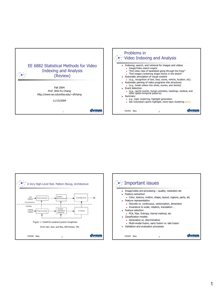
A Very High-Level Stat. Pattern Recog. Architecture Image/video pre-processing – quality, resolution etc � Feature extraction � � Color, texture, motion, shape, layout, regions, parts, etc Feature representation � � Discrete vs. continuous, vectorization, dimension � Invariance to scale, rotation, translation … Feature selection � � PCA, Max. Entropy, Kernel method, etc Classification models � � Generative vs. discriminative � Multi-modal fusion, early fusion vs. late fusion Validation and evaluation processes (From Jain, Duin, and Mao, SPR Review, ’99) � EE6882 - C h ang EE6882 - C h ang 3 4 1

  2. Basic Image/Video Features � Image Features Color (a). SCD (scalable color descriptor) (b). CSD (color structure descriptor) (c). Dominant Color (d). CLD (color layout descriptor) Texture (a). Texture Browsing Descriptor (b). HTD (homogeneous texture descriptor) (c). Edge Histogram Descriptor Motion (a). Motion Activity (b). Motion Trajectory Shape (a). Curvature Scale Space (b). Region moments EE6882 - C h ang EE6882 - C h ang 5 6 Color Histogram Color Space � Feature extraction from color images � Choose color space � Quantize color space to reduce number of colors � brightness varies along the � Represent image color content using color vertical axis histogram � hue varies along the � Feature vector IS the color histogram circumference  = = = 1 if I [ , ] m n r I , [ , ] m n g I , [ , ] m n b ∑∑ R G B � saturation varies along the = h [ , , ] r g b  RGB 0 otherwise  radius m n A color histogram represents the distribution of colors where each histogram bin corresponds to a color is the quantized color space EE6882 - C h ang EE6882 - C h ang 7 8 2

  3. Mohalanobis Metric Histogram Metrics ( ) ( ) 2 T − 1 D = x − x C x − x mah 1 2 x 1 2 ∑   c (1,1) c (1,2) ... c (1, ) d + = − D i i ( , 1) H ( ) j H ( ) j � L 1 distance + 1 i i 1   =  covariance matrix C ... ... ... ... j  x   ∑ c d ( ,1) c d ( ,2) ... c d d ( , ) 2   D i i ( , + 1) = H ( ) j − H ( ) j � L 2 distance 2 i i + 1 N j ∑ =  −   −  − c i j ( , ) x ( ) i m i ( ) x ( ) j m j ( ) N / 1, N number of samples : ∑     ( ) min H ( ), j H ( ) j k k + i i 1 = k 1 � Histogram Intersection j x j x j x j x j x j D = − 1 I   ∑ ∑   o min H ( ), j H ( ) j o o o o o o o oo oo i + 1 i o   o o o o o   j j o o o o o � Quadratic Distance o o ∑∑ ( ) ( ) x i x i x i x i x i = − α − D H ( j ) H ( j ) ( j , j ) H ( j ) H ( j ) 1 c = 1 = − 0 = Q i 1 i + 1 1 1 2 i 2 i + 1 2 c s s = − c s s c s s = i j c s s i j i j i j j j 2 1 2 2 s i , s j : std. deviation α ( j , j ) : correlation between colors j , j e.g. 1-d . � � � � � � 1 2 1 2 j ,j T C =  e | e ...| e  diag ( λ λ , ,..., λ )  e | e ...| e  1 2     x 1 2 d 1 2 d 1 2 d � � � � � � − 1 − 1 T C =  e | e ...| e  ( diag ( λ λ , ,..., λ ))  e | e ...| e      x 1 2 d 1 2 d 1 2 d e 1 e 2 oo o o Projects data to the eigen vectors, divide the sd of o o each eigen dimension, and compute Euclidian distance EE6882 - C h ang 9 Color Coherence Vector Not just  B C B B A A    count of B B C B A A    2 1 2 2 1 1  Color Quantization � More Features to be considered colors, also   B C D B A A   → →  2 2 1 2 1 1 Region Segmentaition  check   B B B A E E     ... ... Labeling adjacency     B B A A E E    B B A A E E    Color 1 2 3 A B C D E α Regions: Color 1 2 1 3 1 Color Co. Vector: 17 15 0 Size 12 15 3 1 5 β 3 0 1 ( ) ( ) ( ) ( ) = α β α β ′ = α β ′ ′ α ′ β ′ G , ,..., , G , ,..., , I 1 1 n n I 1 1 n n n n ∑ ∑ ( ) ( ) ∆ α − α ′ + β − β ′ ∆ α − α ′ + β − β ′ � � G i i i i H i i i i i = 1 i = 1 ∆ > ∆ by triangular inequality G H EE6882 - C h ang 11 3

  4. MPEG-7 Scalable Color Descriptor MPEG-7 Texture Edge Histogram Descriptor + Lowpass coefficient Bin Value 1 + (sum) - ∑ Highpass coefficient Bin Value 2 + (different) Haar Transform Coefficients 16 32 Each image block is then Each Sub-image is 64 partitioned into 2x2 block of Nonlinear Quantization divided into a pixels. The edge detector Original Image fixed number of 256 Histogram values operators are then applied to Linear Quantization 128 divided into 16 blocks. these 2x2 blocks, treating sub-images each block as a pixel and the average intensity as the Filters for edge detection. ∑ corresponding block intensity 256 value. 0 0 2 -2 1 -1 1 1 2 2 -1 -1 0 0 -2 2 1 -1 − 2 − 2 3 bits/bin Scaling Total = 240 bits 5 bins x 16 = 80 bins MPEG-7 Homogeneous Texture descriptor Texture features ω � Fourier Domain Energy Distribution y � Angular features (directionality) φ = ∫∫ 2 V F ( u , v ) dudv θ θ 1 2 ω where , x  v  θ ≤ − 1 ≤ θ tan   1 2  u  ≤ W ≤ 0 1 In a normalized frequency space , the center frequencies of ω y 30 � the feature channels are spread equally in in angular direction � Radial features (coarseness) = ∫∫ r ∈ { 0 , 1 , 2 , 3 , 4 , 5 } such that , where r is angular index with q r = 30 � × r . In 2 V r F ( u , v ) dudv r the radial direction, the center frequencies of the neighboring feature r 1 2 ω = ω − s ∈ 2 , s { 0 , 1 , 2 , 3 , 4 } where , channels are spaced octave apart such that s 0 0 = W 3 / 4 where s is radial index and is the highest center ω ≤ 2 + 2 < r u v r x frequency. The channel index i can be expressed as I = 6 x s + r + 1. 1 2 EE6882 - C h ang EE6882 - C h ang 15 16 4

  5. Curvature Scale Space � Finds curvature zero � How to measure the performance crossing points of the shape’s contour (key points) � Reduces the number of key points step by step, by applying Gaussian smoothing � The position of key points are expressed relative to the length of the contour curve EE6882 - C h ang EE6882 - C h ang 17 18 Evaluation Evaluation Measures Precision Recall Curve = V n 1 " Relevant" P ( P vs R ) 0 " Irrelevant " n = 0 � N - 1 K ranked returned Result N Images in DB R R = A /( A + C ) � Recall ∑ K − 1 � Detection = A V − n 2. Receiver Operating Characteristic (ROC Curve) A vs B n 0 ∑ − K 1 A B = ( 1 − V ) � False Alarms = + P A /( A B ) n n = 0 (hit) 3. Relative Operating Characteristic � Precision ∑ N − 1 = − C ( V ) A n A vs F B (false) � Misses n = 0 = + ∑ N − 1 F B /( B D ) = − − D ( ( 1 V ) ) B = n n 0 4. P value � Fallout ∑ − � Correct Dismissals N 1 = P at cut off k int( V ) k = n n 0 “Returned” “Relevant Ground Truth” ⋅ P R = 5. 3-point P value F 1 + ( P R ) / 2 D A C B = Avg P at R 0 .2 0.5 0.8 � Combined EE6882 - C h ang EE6882 - C h ang 19 20 5

Download Presentation
Download Policy: The content available on the website is offered to you 'AS IS' for your personal information and use only. It cannot be commercialized, licensed, or distributed on other websites without prior consent from the author. To download a presentation, simply click this link. If you encounter any difficulties during the download process, it's possible that the publisher has removed the file from their server.

Recommend


More recommend