1 Mux Representation of Boolean Functions MUX circuit to implement - - PDF document

SLIDE 1

1

ECE 474a/575a Susan Lysecky 1 of 31

ECE 474A/57A Computer-Aided Logic Design

Lecture 11 Binary Decision Diagrams (BDDs)

ECE 474a/575a Susan Lysecky 2 of 31

Boolean Logic Functions Representations

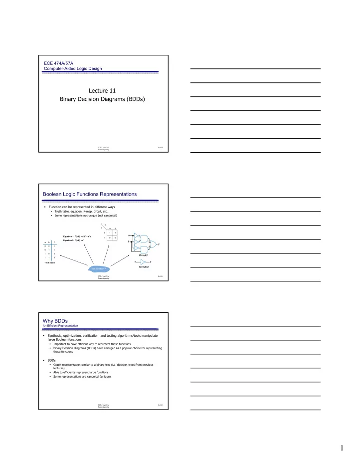
• Function can be represented in different ways
• Truth table, equation, K-map, circuit, etc…
• Some representations not unique (not canonical)

a a b F F Circuit 1 Circuit 2

a 1 1 b 1 1 F 1 1

The function F

Truth table Equation 2: F(a,b) = a’ Equation 1: F(a,b) = a’b’ + a’b 1 1 1 1 F b a ECE 474a/575a Susan Lysecky 3 of 31

Why BDDs

An Efficient Representation

• Synthesis, optimization, verification, and testing algorithms/tools manipulate

large Boolean functions

• Important to have efficient way to represent these functions
• Binary Decision Diagrams (BDDs) have emerged as a popular choice for representing

these functions

• BDDs
• Graph representation similar to a binary tree (i.e. decision trees from previous

lectures)

• Able to efficiently represent large functions
• Some representations are canonical (unique)

SLIDE 2

2

ECE 474a/575a Susan Lysecky 4 of 31

Mux Representation of Boolean Functions

• MUX circuit to implement logic

function S

S(x1, x2, x3) x3 x2 x1 1 MUX 1 1 MUX 1 1 MUX 1 1 MUX x3 x2 x1 S 1 1 1 1 1 1 1 1 1 1 1 1 1 1 1 1 1 S(0, 0, 0) = 1 X3 (0) x2 (0) X1 (0) 1 MUX 1 1 MUX 1 1 MUX 1 1 MUX S(0, 0, 1) = 0 X3 (1) x2 (0) X1 (0) 1 MUX 1 1 MUX 1 1 MUX 1 1 MUX S(0, 1, 0) = 1 X3 (0) x2 (1) X1 (0) 1 MUX 1 1 MUX 1 1 MUX 1 1 MUX S(1, 1, 1) = 0 X3 (1) x2 (1) X1 (1) 1 MUX 1 1 MUX 1 1 MUX 1 1 MUX ECE 474a/575a Susan Lysecky 5 of 31

Mux Representation of Boolean Functions

Relation to BDDs

• Corresponding BDD to implement function S
• One-to-one correspondence to the MUX gates in

the flipped circuit

x3 x2 x1 S 1 1 1 1 1 1 1 1 1 1 1 1 1 1 1 1 1 S(x1, x2, x3) x3 x2 x1 1 MUX 1 1 MUX 1 1 MUX 1 1 MUX Same circuit, just flipped Corresponding BDD 1 x1 x2 x2 x3 S(x1, x2, x3) S(x1, x2, x3) x3 x2 x1 1 MUX 1 1 MUX 1 1 MUX 1 1 MUX ECE 474a/575a Susan Lysecky 6 of 31

Binary Decision Diagram (BDD)

Example 1

• How does it work?
• Line with bubble represent value = 0
• Lines without bubble represent value = 1

x3 x2 x1 S 1 1 1 1 1 1 1 1 1 1 1 1 1 1 1 1 1 1 x1 x2 x2 x3 S(x1, x2, x3) 1 x1 x2 x2 x3 S(0, 0, 0) 1 x1 x2 x2 x3 S(1, 1, 1) 1 x1 x2 x2 x3 S(0, 1, 0) 1 x1 x2 x2 x3 S(0, 0, 1)

SLIDE 3

3

ECE 474a/575a Susan Lysecky 7 of 31

Binary Decision Diagram (BDD)

Edge Notations

• Several ways to represent value = 1 and value = 0
• Bubble vs. Non-bubble line
• Dashed vs. Solid line
• T (then) vs. E (else) labels
• We will adopt T vs. E labels – consistent with most of the book (Hatchel) examples

1 x1 x2 x2 x3 S(x1, x2, x3) 1 x1 x2 x2 x3 S(x1, x2, x3) 1 x1 x2 x2 x3 S(x1, x2, x3) T E T E T E T E ECE 474a/575a Susan Lysecky 8 of 31

Binary Decision Diagram (BDD)

Example 2

• Let’s consider another function

f(a,b,c,d) = abc + b’d + c’d

1 a b b d T E T T E E T E f c c T T E E 1 a b b d T E T T E E T E f c c T T E E What is the value of f(1,0,1,0)? Notice that if a=1 and b=0, the function does not depend on a value for c. 1 a b b d T E T T E E T E f c c T T E E What is the value of f(1,1,0,1)? ECE 474a/575a Susan Lysecky 9 of 31

Ordered Binary Decision Diagram (OBDD)

What is a OBDD?

• Ordered binary decision diagrams ensure the variables appear in

the same order along all paths from the root to the leaves

1 a c c T T T E E E f b T E

Ordering : a ≤ c ≤ b Not ordered

1 a c b T T T E E E f b c T T E E

SLIDE 4

4

ECE 474a/575a Susan Lysecky 10 of 31

Ordered Binary Decision Diagram (OBDD)

Different Ordering Lead to Different Complexity – Example1

• Variable ordering important, may result in a more complex (or simple) BDD
• All three BDDs below represent the same function
• Third ordering (b ≤ c ≤ a ≤ d) optimal because there is exactly one node for

each variable

1 b c d T E T E T E f a T E

Order : b ≤ c ≤ a ≤ d

1 a b b d T E T T E E T E f c c T T E E

Order : a ≤ b ≤ c ≤ d

1 a d d c T E T T E E T E f b b T T E E

Order : a ≤ d ≤ b ≤ c

c T E ECE 474a/575a Susan Lysecky 11 of 31

Ordered Binary Decision Diagram (OBDD)

Different Ordering Lead to Different Complexity – Example 2

• Consider F = ab + cd + ef, again both BDDs represent same function
• Variable order has a large impact on resulting BDD, first variable ordering (a

≤ b ≤ c ≤ d ≤ e ≤ f) yields a much simpler BDD

Order : a ≤ b ≤ c ≤ d ≤ e ≤ f Order : a ≤ c ≤ e ≤ b ≤ d ≤ f

1 a b e d T E T T E E T E f f c T T E E a e c f b b c e e e b b d d f 1 ECE 474a/575a Susan Lysecky 12 of 31

BDDs for Basic Logic Functions

1 a T E f

NOT

a F 1 1

AND

b a F 1 1 1 1 1 1 a b E T T E f

OR

b a F 1 1 1 1 1 1 1 1 a b E E T T f

XOR

b a F 1 1 1 1 1 1 1 a b b E E E T T T f

NAND

b a F 1 1 1 1 1 1 1 f 1 a b E T T E

SLIDE 5

5

ECE 474a/575a Susan Lysecky 13 of 31

Formal Definition of BDDs

• A BDD is a direct acyclic graph (DAG) representing a

multiple-output switching function F

• Nodes are partitioned into three subsets
• Function node
• Represents the function symbol (f)
• Indegree = 0
• Outdegree = 1
• Internal node
• Represents variable in function (a, b, c, d)
• Indegree ≥ 1
• Outdegree = 2
• Terminal node
• Represents a value (1 or 0)
• Indegree ≥ 1
• Outdegree = 0

1 b c d T E T E T E f a T E Function node Internal nodes Terminal nodes ECE 474a/575a Susan Lysecky 14 of 31

Formal Definition of BDDs

• A BDD definition (cont’)
• Three types of edges
• Incoming edge
• From the function node and defines function
• T edge
• From an internal node and represents when

the corresponding variable is 1

• E edge
• From an internal node and represents when

the corresponding variable is 0

1 b c d T E T E T E f a T E Incoming edge E edge T edge ECE 474a/575a Susan Lysecky 15 of 31

Formal Definition of BDDs

• A BDD definition (cont’)
• The function f represented by a BDD is

defined as follows

• The function of the terminal node is a

constant value (1 or 0)

• The function of a T edge is the function of

the head node

• The function of a E edge is the complement
• f the function of the node
• The function of a node v is given by vfT +

v’fE, when fT is the function of the T edge and fE is the function of the E edge

• The function of the function node is the

function of it’s outgoing edge 1 b c d T E T E T E f a T E Function of the function node is the function of it’s outgoing edge Function of this T edge is a Function of this terminal node is 1 Function of this terminal node is 0 Function of this E edge is a’

SLIDE 6

6

ECE 474a/575a Susan Lysecky 16 of 31

BDD Canonical Form

• BDDs are canonical (unique) for a representation of

F given a variable ordering if

• All internal nodes are descendants of some node
• There are no isomorphic subgraphs
• For every node fT ≠ fE

1 b d E T T E f 1 c E T d T E 1 Isomorphic Two graphs are isomorphic if there is a one-to-one correspondence between their vertices and there is an edge between two vertices of one graph if and only if there is an edge between the two corresponding vertices in the other graph English – same subgraph - all vertices the same, all edges between vertices the same Isomorphic subgraphs ECE 474a/575a Susan Lysecky 17 of 31

Building BDDs For a Function F

• How do I build a BDD given a function F ?
• Recursive use of Shannon’s Expansion Theorem
• F = aFa + a’Fa’
• We can keep applying expansion theorem,

eventually we reach the unique canonical form , which uses only minterms F = a’b + abc’ + a’b’c F = a(bc’) + a’(b+b’c) Fa = (bc’) Fa also called the cofactor of F w.r.t. (with respect to) a Fa’ = (b+b’c) F = a’b + abc’ + a’b’c F = cFc + c’Fc’ F expanded w.r.t to c F = c(a’b + a’b’) + c’(a’b + ab) F = a’b + abc’ + a’b’c F = bFb + b’Fb’ F expanded w.r.t to b F = b(a’+ ac’) + b’(a’c)

ECE 474a/575a Susan Lysecky 18 of 31

Building BDDs - Exercise 1

• Build a BDD for f = abc + ab’c + a’bc’ + a’b’c’
• Use the variable ordering a ≤ b ≤ c

f

Compute cofactors of f with respect to a (first variable in ordering) f = abc + ab’c + a’bc’ + a’b’c’ fa’ = bc’ + b’c’

a E T f

fa fa’

partial expansion with respect to a

fa = bc + b’c

SLIDE 7

7

ECE 474a/575a Susan Lysecky 19 of 31

Building BDDs - Exercise 1

• Build a BDD for f = abc + ab’c + a’bc’ + a’b’c’
• Use the variable ordering a ≤ b ≤ c

f

Compute cofactors of fa and fa’ with respect to b (second variable in ordering) fa = bc + b’c fa’ = bc’ + b’c’ (fa)b’ = fab’ = c

a E T f partial expansion with respect to b

(fa)b = fab = c

b E T

fab fab’

(fa’)b’ = fa’b’ = c’ (fa’)b = fa’b = c’

b E T

fa’b fa’b’

a E T

fa fa’

ECE 474a/575a Susan Lysecky 20 of 31

Building BDDs - Exercise 1

• Build a BDD for f = abc + ab’c + a’bc’ + a’b’c’
• Use the variable ordering a ≤ b ≤ c

f

Compute cofactors of fab, fab’, fa’b, fa’b’ with respect to c (third variable in ordering) fab’ = c fab = c fa’b’ = c’ fa’b = c’

expansion with respect to c, final BDD

fabc’ = 0 fabc = 1

a E T f b E T b E T c E T 1

fab’c = 1 fab’c’ = 0

c E T 1

fa’bc = 0 fa’bc’ = 1

c E T 1

fa’b’c = 0 fa’b’c’ = 1

c E T 1 a E T b E T

fab fab’

b E T

fa’b fa’b’

ECE 474a/575a Susan Lysecky 21 of 31

Building BDDs - Exercise 1

• f = abc + ab’c + a’bc’ + a’b’c’

a E T f b E T b E T c E T c E T c E T c E T 1 1 1 1

Does it work? f b 1 1 1 1 c 1 1 1 1 a 1 1 1 1 1 1 1 1

SLIDE 8

8

ECE 474a/575a Susan Lysecky 22 of 31

Building BDDs - Exercise 2

• Build a BDD for f = abc + b’d + c’d
• Use the variable ordering b ≤ c ≤ d ≤ a

f

Compute cofactors of f with respect to b (first variable in ordering) f = abc + b’d + c’d fb’ = d + c’d

b E T f

fb fb’

partial expansion with respect to b

fb = ac + c’d

ECE 474a/575a Susan Lysecky 23 of 31

Building BDDs - Exercise 2

• Build a BDD for f = abc + b’d + c’d
• Use the variable ordering b ≤ c ≤ d ≤ a

Compute cofactors of fb and fb’ with respect to c (second variable in ordering) fb = ac + c’d fb’ = d + c’d

b E T f

fb fb’

b E T f

fbc

c E T

fbc’ = fb’c = fb’c’

equivalent cofactors, we can create a single node (reduced)

fb’c = d fb’c’ = d

fb’c

c E T

fb’c’ fbc

c E T

fbc’

b E T f

fbc = a fbc’ = d

partial expansion with respect to c ECE 474a/575a Susan Lysecky 24 of 31

Building BDDs - Exercise 2

• Build a BDD for f = abc + b’d + c’d
• Use the variable ordering b ≤ c ≤ d ≤ a

Compute cofactors of fbc’, fb’c, and fb’c’ with respect to d (third variable in ordering) fbc’ = fbc’ = fb’c’ = d

b E T f

fbc

c E T

fbc’ = fb’c = fb’c’

fbc’d = fbc’d = fb’c’d = 1 fbc’d’ = fbc’d’ = fb’c’d’ = 0

b E T f

fbc

c E T d E T 1 partial expansion with respect to d

SLIDE 9

9

ECE 474a/575a Susan Lysecky 25 of 31

Building BDDs - Exercise 2

• Build a BDD for f = abc + b’d + c’d
• Use the variable ordering b ≤ c ≤ d ≤ a

Compute cofactors of fbc with respect to a (fourth variable in ordering)

b E T f

fbc

c E T

fbc = a

d E T 1 b E T f c E T d E T 1

fbca = 1 fbca’ = 0

a E T expansion with respect to a, final BDD ECE 474a/575a Susan Lysecky 26 of 31

Building BDDs - Exercise 2

• Build a BDD for f = abc + b’d + c’d

Does it work?

b E T f c E T d E T 1 a E T

f b 1 1 1 1 c 1 1 1 1 d 1 1 1 1 a 1 1 1 1 1 1 1 1 1 1 1 1 1 1 1 1 1 1 1 1 1 1 1 1 1 1 1 1

ECE 474a/575a Susan Lysecky 27 of 31

BDD to Boolean Function – Exercise 1

• Can we go from a BDD to a Boolean function ?
• Sum all paths from function node to terminal nodes

b E T f c E T d E T 1 a E T

F = bca + bc’d + b’d = aFa + a’Fa’ = a(1) + a(0) = a + 0 = a = cFc + c’Fc’ = c(a) + c’(d) = ca + c’d = bFb + b’Fb’ = b(ca + c’d) + b’(d) = bca + bc’d + b’d = d

SLIDE 10

10

ECE 474a/575a Susan Lysecky 28 of 31

BDD to Boolean Function – Exercise 2

• Another Example

a E T f b E T 1 c E T

F = abc’ + ab’ + a’ = c’ = bFb + b’Fb’ = b(c’) + b’(1) = bc’ + b’ = aFa + a’Fa’ = a(bc’ + b’) + a’(1) = abc’ + ab’ + a’

ECE 474a/575a Susan Lysecky 29 of 31

Reducing BDDs

a E T f b E T b E T c E T 1 c E T 1 c E T 1 c E T 1

isomorphic subgraphs

a E T f b E T b E T c E T 1 c E T 1 c E T 1 a E T f b E T c E T 1 c E T 1 c E T 1

• When building BDDs, result not always reduced (Example 1 - slide 19)
• We have isomorphic subgraphs, potential for reduction
• Transform a non-reduced BDD into a reduced BDD by iteratively applying
• Identify isomorphic subgraphs
• Remove redundant nodes
• A ordered reduced BDD (ROBDD) is unique so we have a canonical form

Fb = Fb’ (redundant node)

ECE 474a/575a Susan Lysecky 30 of 31

Reducing BDDs

Example 2

isomorphic subgraphs

a T f b E T c E T 1 c E T 1 E c E T 1 a T f b E T c E T 1 E c E T 1 a T f E c E T 1 c E T 1

• Let’s try to reduce and OBDD
• Iterative apply
• Identify isomorphic subgraphs
• Remove redundant nodes

Fb = Fb’ (redundant node)

SLIDE 11

11

ECE 474a/575a Susan Lysecky 31 of 31

Summary, and then some…

• Binary Decision Diagrams (BDDs)
• Efficient mechanism to representation of Boolean functions in terms of memory and

CPU

• Translating function→BDD and BDD→function
• Importance of variable ordering
• Method to reduced OBDDs, getting a ROBDD
• We said that BDDs can be efficiently stored and manipulated – HOW?
• Refer to handwritten notes
• Supplemental materials attached

ECE 474a/575a Susan Lysecky 32 of 31

ITE Operator

Two argument operators expressed in terms of ITE

F F F 0011 ITE(F, G’, 0) FG’ F > G 0010 ITE(F, G, 0) FG AND(F, G) 0001 0000 G G G 0101 ITE(F, 0, G) F’G F < G 0100 ITE(F, 1, G) F + G OR(F, G) 0111 ITE(F, G’, G) F ⊕ G XOR(F, G) 0110 ITE(F, G, G’) (F ⊕ G)’ XNOR(F, G) 1001 ITE(F, 0, G’) (F + G)’ NOR(F, G) 1000 ITE(F, 1, G’) F + G’ F ≥ G 1011 ITE(G, 0, 1) G’ NOT(G) 1010 ITE(F, G, 1) F’ + G F ≤ G 1101 ITE(F, 0, 1) F’ NOT(F) 1100 ITE(F, G’, 1) (FG)’ NAND(F, G) 1110 1 1 1 1111

Equivalent Form Expression Name Table

ECE 474a/575a Susan Lysecky 33 of 31

ITE Algorithm

ITE(F, G, H) = FG + F’H = v(FG + F’H)v + v’(FG + F’H)v’ = v(FvGv + F’vHv) + v’(Fv’Gv’ + F’v’Hv’) = ITE( v, ITE(Fv, Gv, Hv), ITE(Fv’, Gv’, Hv’) )

• Terminal cases are as follows
• Most standard manipulation of BDDs can be done with ITE
• Algorithm recursive, based on formulation where v is the top variable of F, G, H

ITE(1, F, G) = ITE(0, G, F) = ITE(F, 1, 0) = ITE(G, F, F) = F

SLIDE 12

12

ECE 474a/575a Susan Lysecky 34 of 31

Pseduo-code of the ITE Algorithm

ITE(F, G, H){ (result, terminal_case) = TERMINAL_CASE(F, G, H) if (terminal_case) return (result) (result, in_computed_table) = COMPUTED_TABLE_HAS_ENTRY(F, G, H) if (in_computed_table) return (result) v = TOP_VARIABLE(F, G, H) T = ITE(Fv, Gv, Hv) E = ITE(Fv’, Gv’, Hv’) R = FIND_OR_ADD_UNIQUE_TABLE(v, T, E) INSERT_COMPUTED_TABLE((F, G, H), R) return (R) } // did we find a terminal case? // have we already calculated this value? // recursively calculate this value // see if subtree already present // record the calculated value