1 II.A. Extended Form Equations (contd.) Extended Form Equations - - PDF document

1

1

Multiple Equilibria and Sunspots in a Security Multiple Equilibria and Sunspots in a Security Market with Investment Restrictions Market with Investment Restrictions

Suleyman Suleyman Basak Basak, David Cass, Juan M. Licari, Anna , David Cass, Juan M. Licari, Anna Pavlova Pavlova

I. I. Motivation and Main Results Motivation and Main Results II. II. A Model of Financial Equilibrium (FE) with Investment A Model of Financial Equilibrium (FE) with Investment Restrictions Restrictions III.

• III. The Simplest Example: Multiple Equilibria and Sunspots

The Simplest Example: Multiple Equilibria and Sunspots IV.

• IV. Some Extensions

Some Extensions V. V. Further Research Further Research

LBS LBS UPenn UPenn UPenn UPenn MIT MIT

2

I.

• I. Motivation and Main Results

Motivation and Main Results

• A. History of the project
• B. Multiple Equilibria/Sunspot Equilibria: applied theory

(Finance – asset pricing) vs theory (Economics – financial equilibrium)

• C. Main Results about the Structure of FE in the Simplest

Example: Multiple Equilibria/Sunspot Equilibria

3

• Two specializations of FE:

(a) “Trees:” stocks with the properties that (i) the return from stock g g is in terms of good g g, and (ii) endowments consist wholly of stocks (and possibly bonds, also having good-specific returns) (b) “Logs:” log-linear expected utility

• FE is described by the equations representing household
• ptimization (first-order conditions, budget constraints, and

investment restrictions) and market clearing conditions

• Glossary

II.

• II. A Model of Financial Equilibrium with Investment

A Model of Financial Equilibrium with Investment Restrictions Restrictions

4

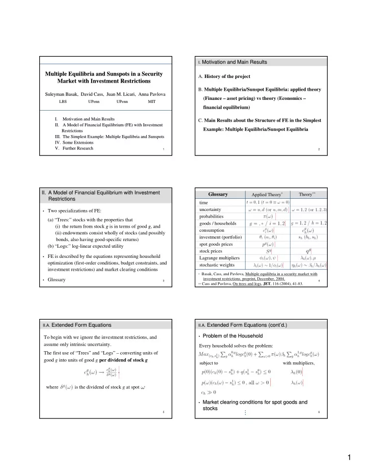
Glossary Glossary

time uncertainty probabilities goods / households consumption investment (portfolio) spot goods prices stock prices Lagrange multipliers stochastic weights Applied Theory* Theory**

* Basak, Cass, and Pavlova, Multiple equilibria in a security market with

investment restrictions, preprint, December, 2004.

** Cass and Pavlova, On trees and logs, JET, 116 (2004), 41-83. 5

II.A. II.A. Extended Form Equations

Extended Form Equations To begin with we ignore the investment restrictions, and assume only intrinsic uncertainty. The first use of “Trees” and “Logs” – converting units of good g into units of good g per dividend of stock g where is the dividend of stock g at spot ,

6

• Problem of the Household

Problem of the Household Every household solves the problem:

II.A. II.A. Extended Form Equations (cont’d.)

Extended Form Equations (cont’d.)

subject to with multipliers,

• Market clearing conditions for spot goods and

Market clearing conditions for spot goods and stocks stocks

. . .

2

7

II.A. II.A. Extended Form Equations (cont’d.)

Extended Form Equations (cont’d.)

. . . . . .

where

8

II.B. II.B. Reduced Form Equations

Reduced Form Equations The second use of “Trees” and “Logs” – reducing the number of variables and equations We can use the previous equations to simplify the system to consist of just the spot goods price equations, no-arbitrage conditions, budget constraints, and stock market clearing

• conditions. At this point, it is convenient to replace the Lagrange

multipliers by the stochastic weights . After some manipulation, this yields:

9

II.B. II.B. Reduced Form Equations (cont’d.)

Reduced Form Equations (cont’d.) SGP’s NAC’s BC’s

good eqs. bad eqs.

10

II.B. II.B. Reduced Form Equations (cont’d.)

Reduced Form Equations (cont’d.) Note that (1) By the analogue of Walras’ law, Mr. H’s budget constraints are redundant, and (2) For the purposes of analysis, the variables and equations can be reduced even further by normalizing prices, say, by setting , all , and then (i) substituting for spot goods prices, and (ii) using Ms. 1’s NAC’s, substituting for stock prices in the remaining NAC’s. This leaves only , , , and , , as variables.

11

III.

• III. The Leading Example:

The Leading Example: 2 states, goods, and households

2 states, goods, and households Notice specially that, since there are equal number of states and stocks, the stock market is potentially complete. For simplicity (and without any loss of generality), we take and relabel , , with , and We establish, first, a multiplicity of equilibria, then second (based on the same technique), an abundance of sunspot equilibria – some of which are especially interesting from an “applied” perspective. . all , ω

12

III.A. III.A. A Specific Investment Restriction

A Specific Investment Restriction

• r

with Suppose that Mr. 2 faces the additional constraint , (now) relative price , and associated . multiplier

3

13

Adding the constraint entails two modifications of the reduced form equations: First, the term is added to the right hand side of Mr. 2’s NAC for stock 2, and second, the complementary slackness condition is added to his first-order conditions.

III.A. III.A. A Specific Investment Restriction (cont’d)

A Specific Investment Restriction (cont’d)

14

III.A. III.A. A Specific Investment Restriction (cont’d)

A Specific Investment Restriction (cont’d) This leads to our first main result, based on distinguishing the second period budget constraints from the rest of the reduced form equations, the singular equations (TSE) from the regular equations (TRE) (this labeling reflects the fact that the reduced form equations have an especially critical point – which will be formally described if time permits).

15

III.A. III.A. A Specific Investment Restriction (cont’d)

A Specific Investment Restriction (cont’d) Proposition 1. Proposition 1. Assume that , . Then, there are two cases to consider. Case 1. TRE have a unique solution with , all , so that is colinear to , all . In particular, this implies that TSE reduce to a single equation which has a one- dimensional continuum of solutions s.t. , and

.

16

Case 2.

III.A. III.A. A Specific Investment Restriction (cont’d)

A Specific Investment Restriction (cont’d) There is an open interval with s.t., for , TRE have exactly two distinct solutions with, for example, . (Here and after, it is convenient to utilize the so-called applied theory notation [sic]). Proposition 1. (cont’d) Proposition 1. (cont’d)

17

III.A. III.A. A Specific Investment Restriction (cont’d)

A Specific Investment Restriction (cont’d) Moreover, TSE have a unique solution independent of the stochastic weights We emphasize that this example is very robust. The results we describe obtain on an open set of all the parameters of the model, including . . //

18

For this analysis, we ignore the investment restriction itself and elaborate the analysis of local perturbations of TRE (still including as a variable) around the “stationary” solution , all , in order to derive properties of their global

• solutions. The basic rationale is that if , then we can

“tailor” many investment restrictions which depend on endogenous variables (when they are specified in parametric form). In fact, this can be done for the specific investment restriction introduced in the preceding section – as illustrated in Fig. 1 below.

III.B. III.B. An Abstract Investment Restriction

An Abstract Investment Restriction

4

19

III.B. III.B. An Abstract Investment Restriction (cont’d)

An Abstract Investment Restriction (cont’d) Let represent TRE, where (the “dependent” variables), (the “independent” variable), , and .

20

III.B. III.B. An Abstract Investment Restriction (cont’d)

An Abstract Investment Restriction (cont’d) Proposition 2. Proposition 2. Under the same hypotheses as in Proposition 1, there is a mapping s.t. , for , (i) and , and (ii) and .

21

III.B. III.B. An Abstract Investment Restriction (cont’d)

An Abstract Investment Restriction (cont’d)

• Remark. In fact, while

, and (so that for the variable , we have while ). Applying Proposition 2 for the specific investment restriction introduced earlier yields Proposition 1, as illustrated in Figure 1.

22

Figure 1. Relating the local and global results Figure 1. Relating the local and global results

23

III.B. III.B. An Abstract Investment Restriction (cont’d)

An Abstract Investment Restriction (cont’d) A very important aspect of both Propositions is that if (which must be the case when ), then Rank = 2 and

• 1

is independent of , Both this critical property of TSE and the local analysis of TRE appear to be quite generalizable. .

24

Interpretation of the Propositions Concerning Multiple

• Equilibria. There are two types of equilibria, Pareto efficient

(E-type) and Pareto inefficient (I-type). For the E-type, there is a continuum of equilibria, but in which spot goods prices and allocations are identical. Moreover, the asset market is

• incomplete. For the I-type, there are exactly two distinct

equilibria, but in which the portfolio strategies are identical (in a T-period environment with T>2, this means that investors follow a buy-and-hold strategy). Moreover, the asset market is complete.

III.B. III.B. An Abstract Investment Restriction (cont’d)

An Abstract Investment Restriction (cont’d)

5

25

Suppose now that, in addition to intrinsic uncertainty , there is also extrinsic uncertainty so that overall uncertainty is , with , . Consider the extreme case where . Then Proposition 2 obtains as stated. More generally, for (the “independent” variables now), there will be a 2-dimensional manifold of sunspot equilibria, while the nonsunspot equilibria correspond to the restriction , .

III.C. III.C. Sunspot Equilibria

Sunspot Equilibria , ,b g = σ

26

III.C. III.C. Sunspot Equilibria (cont’d)

Sunspot Equilibria (cont’d) Interpretation of the Proposition 2 (taken as) Concerning Sunspot Equilibria. Say that a “sunspot realization matters” if, conditional on its realization, spot good prices do not smooth consumption, i.e., . (Note that if a sunspot realization doesn’t matter [resp. does matter] then the corresponding conditional allocation is [resp. isn’t] Pareto

• ptimal). There are sunspot equilibria in which sunspots don’t

matter when but do matter when , g = σ

. b = σ

27

IV.

• IV. Some Extensions

Some Extensions These are more or less in order of decrease in our level of

• understanding. Their common feature is that each appears

amenable to local analysis.

• 3 intrinsic states of the world and 2 goods
• T >2 Periods
• More than 2 (intrinsic or extrinsic) states and 2 goods

. . . . . . . . .

28

V.

• V. Further Research

Further Research

• More than 2 households
• Robustness (more than simply parametric):

Beyond the forest (aka trees) Beyond the mill (aka logs) – the most problematic, but also the most interesting – intuition is from the textbook example illustrated in Figure 2.

29

Figure 2. Robustness of utility functions Figure 2. Robustness of utility functions The Walrasian model with G=H=2, log-linear utility functions, with , and total endowments (1,1)

Slope: Slope: