[PDF] - 1 Example: a :1/ 2, b :1/ 4, c d , :1/8 How are the trees PDF Document

SLIDE 1

1

DL - 2004 Compression – Beeri/Feitelson 1

Compression הסיחד

Introduction
Information theory
Text compression
IL compression

DL - 2004 Compression – Beeri/Feitelson 2

General: Compression methods depend on data characteristic there is no universal (best) method

Requirements:

text, EL’s: lossless
images – may be lossy
efficiency --

how may bits per byte of data?

(often in percentage)

coding should be fast, decoding superfast

DL - 2004 Compression – Beeri/Feitelson 3

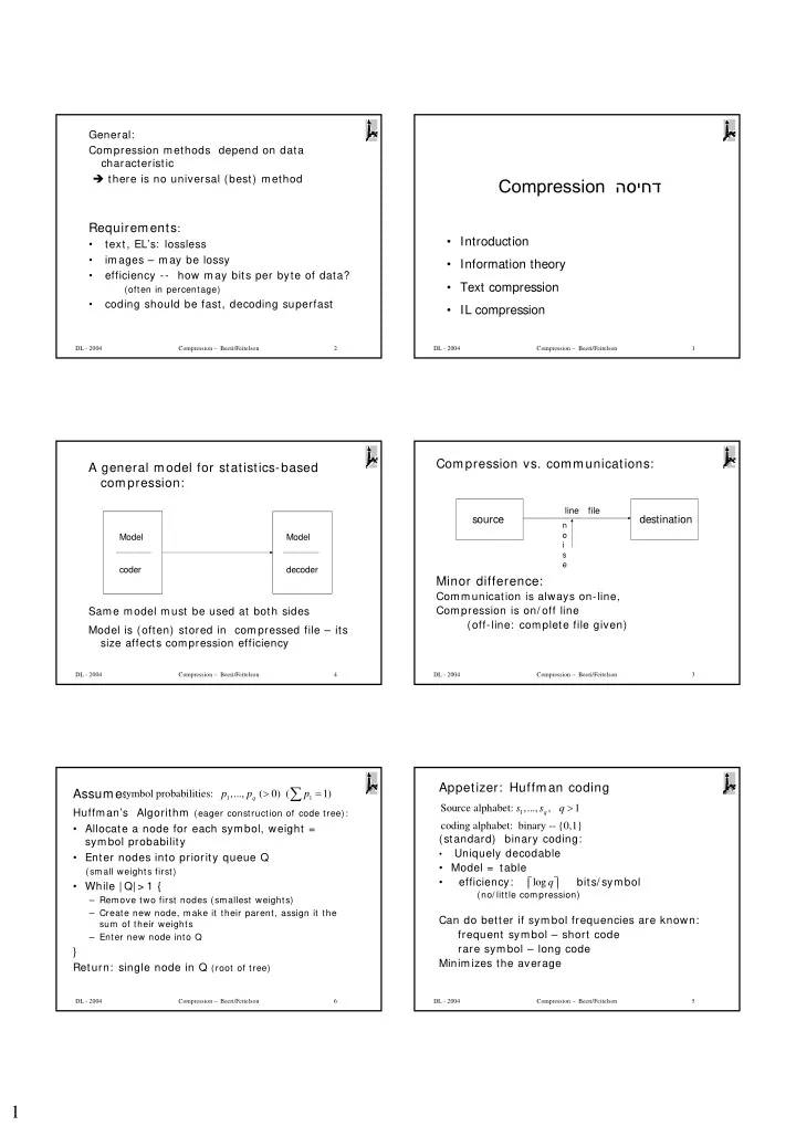
Compression vs. communications: Minor difference:

Communication is always on-line, Compression is on/ off line (off-line: complete file given) source destination

file line

n

i

s e

DL - 2004 Compression – Beeri/Feitelson 4

A general model for statistics-based compression:

Same model must be used at both sides Model is (often) stored in compressed file – its size affects compression efficiency

Model coder Model decoder

DL - 2004 Compression – Beeri/Feitelson 5

Appetizer: Huffman coding

(standard) binary coding:

Uniquely decodable
Model = table
efficiency: bits/ symbol

(no/ little compression)

Can do better if symbol frequencies are known: frequent symbol – short code rare symbol – long code Minimizes the average

1

Source alphabet: ,..., , 1 coding alphabet: binary -- {0,1}

q

s s q > logq    

DL - 2004 Compression – Beeri/Feitelson 6

Assume:

Huffman’s Algorithm (eager construction of code tree):

Allocate a node for each symbol, weight =

symbol probability

Enter nodes into priority queue Q

(small weights first)

While | Q| > 1 {

– Remove two first nodes (smallest weights) – Create new node, make it their parent, assign it the sum of their weights – Enter new node into Q

} Return: single node in Q (root of tree)

1 1

symbol probabilities: ,..., ( 0) ( 1)

q

p p p > =

∑

SLIDE 2

2

DL - 2004 Compression – Beeri/Feitelson 7

Example:

Q: { }

1/4

:1/ 2, :1/ 4, , :1/8 a b c d

1/8 1/4 1/2 1/8 1/8 1/8 1/4 1/2 1 1/2 1/2 1/4 1

DL - 2004 Compression – Beeri/Feitelson 8

How are the trees used?

Coding: for each symbol s, output binary path from root to leaf(s) Decoding: read incoming stream of bits, follow path from root of tree. When leaf(s) reached,

utput s, and return to root.

Common model (stored on both sides) : the tree

DL - 2004 Compression – Beeri/Feitelson 9

Expected cost bits/ symbol:

Binary: Huffman : In example: binary: 2 Huffman : 1/ 2x1 + ¼ x2 + 1/ 8x3 + 1/ 8x3 = 1.75 Q: what would be the tree and cost for: 5/ 12, 1/ 3, 1/ 6, 1/ 12 ? log q     ( length of path from root to leaf( ))

i i i i

p l l s =

∑

DL - 2004 Compression – Beeri/Feitelson 10

A note on Huffman trees:

The algorithm is non-deterministic:

In each step, either node can be the left child of

new parent If two children of a node are exchanged, result is also a Huffman tree Closure under rotation w.r.t nodes

Consider 0.4, 0.2, 0.2, 0.1, 0.1

after 1st step, 2 out of 3 nodes are selected There are many Huffman trees for a given probability distribution

DL - 2004 Compression – Beeri/Feitelson 11

Concepts:

variable length code: (e.g. Huffman) uniquely decodable code: each legal code sequence is generated by a unique source sequence instantaneous/ prefix code ידיימ end of code of each symbol can be recognized Examples: 0, 010, 01, 10 10, 00, 11, 110 0, 10, 110, 111 (Huffman of example) (comma code) 0, 01, 011, 111 (inverted comma code)

DL - 2004 Compression – Beeri/Feitelson 12

A prefix code = binary tree Every binary tree with q leaves is a prefix code for q symbols, lengths of code words = lengths of paths Kraft inequality: Exists a q-leaf tree with path lengths iff = 1 iff tree is complete

1,..., q

l l

2 1

i

l − ≤

∑

SLIDE 3

3

DL - 2004 Compression – Beeri/Feitelson 13

Proof :

assume exists a tree T Take T’ to be the full tree of depth The number of its leaves: A leaf of T, at distance from root has leaves of T’ under it Sum on all leaves of T:

Full: all paths same length

max( )

i

l l = 2l

i

l 2

i

l l −

l

i

l l −

i

l T 2 2 2 1

i i

l l l l − −

≤ ⇒ ≤

∑ ∑

DL - 2004 Compression – Beeri/Feitelson 14

If T is not complete (every node has 0/ 2 children) it has a node with a single child Can be “shortened” new tree still satisfies hence given tree must satisfy Only complete trees have equality Comment: In general a prefix code that is not a complete tree is dominated by a tree with smaller cost From now: tree are complete

2 1

i

l − ≤

∑

2 1

i

l − <

∑

DL - 2004 Compression – Beeri/Feitelson 15

: Assume

Lemma: if Replace these two by their sum (hence q-1 lengths) and use induction Assume must the tree be complete?

2 1

i

l − ≤

∑

max( ) then s.t. =

i j j k

l l k j l l = ∃ ≠

2 1

i

l − =

∑

DL - 2004 Compression – Beeri/Feitelson 16

MacMillan Theorem :

exists a uniquely decodable code with lengths iff Corollary: when there is a uniquely decodeable code, there is also a prefix code (same cost) No need to think about the first class

1,..., q

l l

2 1

i

l − ≤

∑

Uniquely decodable prefix

DL - 2004 Compression – Beeri/Feitelson 17

On optimality of Huffman:

Cost of a tree/ code T: L(T) = Claim: if a tree T does not satisfy then it is dominated by a tree with smaller cost Claim: for any T, Proof: can assume T satisfies (* ) Use induction: Q= 2: both trees have lengths 1,1

i i

p l

∑

1 1

(*) ... ...

q q

p p l l ≥ ≥ ⇒ ≤ ≤

Huff

L(T ) L(T) ≤

DL - 2004 Compression – Beeri/Feitelson 18

Q> 1: In Huffman tree, there are two maximal paths that end in sibling nodes In T, the paths for last two symbols are longest

(by (* )) but their ends may not be siblings

But, T is complete, hence the leaf with has a sibling with same length; exchange with the leaf corresponding to Now, in both trees, these two longest paths can be replaced by their parents Case of q-1 (induction hypothesis)

q

l

1 q

l −

SLIDE 4

4

DL - 2004 Compression – Beeri/Feitelson 19

Summary:

Huffman trees are optimal hence satisfy (* )
Any two Huffman trees have equal costs
Huffman trees have min cost among all trees