Conjugate prior summary Distribution Likelihood p ( x | ) Prior p ( - - PowerPoint PPT Presentation

Conjugate prior summary

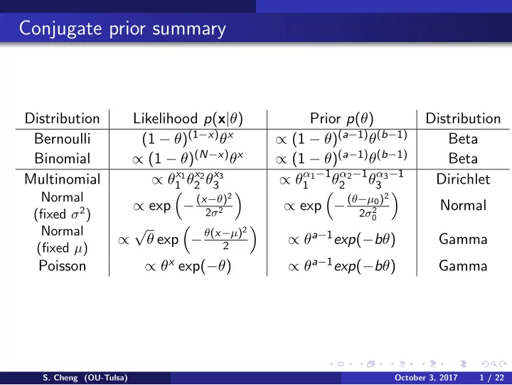
Distribution Likelihood p(x|θ) Prior p(θ) Distribution Bernoulli (1 − θ)(1−x)θx ∝ (1 − θ)(a−1)θ(b−1) Beta Binomial ∝ (1 − θ)(N−x)θx ∝ (1 − θ)(a−1)θ(b−1) Beta Multinomial ∝ θx1

1 θx2 2 θx3 3

∝ θα1−1

1

θα2−1

2

θα3−1

3

Dirichlet

Normal (fixed σ2)

∝ exp

• − (x−θ)2

2σ2

• ∝ exp
• − (θ−µ0)2

2σ2

• Normal

Normal (fixed µ)

∝ √ θ exp

• − θ(x−µ)2

2

• ∝ θa−1exp(−bθ)

Gamma Poisson ∝ θx exp(−θ) ∝ θa−1exp(−bθ) Gamma

• S. Cheng (OU-Tulsa)

October 3, 2017 1 / 22

Lecture 7 Constraint optimization

An example

Simple economy: m prosumers, n different goods1 Each individual: production pi ∈ Rn , consumption ci ∈ Rn Expense of producing “p” for agent i = ei(p) Utility (happiness) of consuming “c” units for agent i = ui(c) Maximize happiness max

pi,ci

• i

(ui(ci) − ei(pi)) s.t.

• i

ci =

• i

pi

1Example borrowed from the first lecture of Prof Gordon’s CMU CS 10-725

• S. Cheng (OU-Tulsa)

October 3, 2017 2 / 22

Lecture 7 Constraint optimization

Walrasian equilibrium

max

pi,ci

• i

(ui(ci) − ei(pi)) s.t.

• i

ci =

• i

pi Idea: introduce price λj to each good j. Let the market decide

Price λj ↑ : consumption of good j ↓, production of good j ↑ Price λj ↓ : consumption of good j ↑, production of good j ↓ Can adjust price until consumption = production for each good

• S. Cheng (OU-Tulsa)

October 3, 2017 3 / 22

Lecture 7 Constraint optimization

Algorithm: tˆ atonnement

Assume that the appropriate prices are found, we can ignore the equality constraint, then the problem becomes max

pi,ci

• i

(ui(ci) − ei(pi)) ⇒

• i

max

pi,ci (ui(ci) − ei(pi))

So we can simply optimize production and consumption of each individual independently Algorithm 1 tˆ atonnement

1: procedure FindBestPrices 2:

λ ← [0, 0, · · · , 0]

3:

for k = 1, 2, · · · do

4:

Each individual solves for its ci and pi for the given λ

5:

λ ← λ + δk

• i(ci − pi)
• S. Cheng (OU-Tulsa)

October 3, 2017 4 / 22

Lecture 7 Constraint optimization

Lagrange multiplier

Problem max

x

f (x) g(x) = 0 Consider L(x, λ) = f (x) − λg(x) and let ˜ f (x) = minλ L(x, λ).

• S. Cheng (OU-Tulsa)

October 3, 2017 5 / 22

Lecture 7 Constraint optimization

Lagrange multiplier

Problem max

x

f (x) g(x) = 0 Consider L(x, λ) = f (x) − λg(x) and let ˜ f (x) = minλ L(x, λ). Note that ˜ f (x) =

• f (x) if g(x) = 0

−∞ otherwise

• S. Cheng (OU-Tulsa)

October 3, 2017 5 / 22

Lecture 7 Constraint optimization

Lagrange multiplier

Problem max

x

f (x) g(x) = 0 Consider L(x, λ) = f (x) − λg(x) and let ˜ f (x) = minλ L(x, λ). Note that ˜ f (x) =

• f (x) if g(x) = 0

−∞ otherwise Therefore, the problem is identical to maxx ˜ f (x) or max

x

min

λ (f (x) − λg(x)),

where λ is known to be the Lagrange multiplier.

• S. Cheng (OU-Tulsa)

October 3, 2017 5 / 22

Lecture 7 Constraint optimization

Lagrange multiplier (con’t)

Assume the optimum is a saddle point, max

x

min

λ (f (x) − λg(x)) = min λ max x (f (x) − λg(x)),

the R.H.S. implies ∇f (x) = λ∇g(x)

• S. Cheng (OU-Tulsa)

October 3, 2017 6 / 22

Lecture 7 Constraint optimization

Inequality constraint

Problem max

x

f (x) g(x) ≤ 0 Consider ˜ f (x) = minλ≥0(f (x) − λg(x)),

• S. Cheng (OU-Tulsa)

October 3, 2017 7 / 22

Lecture 7 Constraint optimization

Inequality constraint

Problem max

x

f (x) g(x) ≤ 0 Consider ˜ f (x) = minλ≥0(f (x) − λg(x)), note that ˜ f (x) =

• f (x)

if g(x) ≤ 0 −∞

• therwise
• S. Cheng (OU-Tulsa)

October 3, 2017 7 / 22

Lecture 7 Constraint optimization

Inequality constraint

Problem max

x

f (x) g(x) ≤ 0 Consider ˜ f (x) = minλ≥0(f (x) − λg(x)), note that ˜ f (x) =

• f (x)

if g(x) ≤ 0 −∞

• therwise

Therefore, we can rewrite the problem as max

x

min

λ≥0(f (x) − λg(x))

• S. Cheng (OU-Tulsa)

October 3, 2017 7 / 22

Lecture 7 Constraint optimization

Inequality constraint (con’t)

Assume max

x

min

λ≥0(f (x) − λg(x)) = min λ≥0 max x (f (x) − λg(x))

The R.H.S. implies ∇f (x) = λ∇g(x)

• S. Cheng (OU-Tulsa)

October 3, 2017 8 / 22

Lecture 7 Constraint optimization

Inequality constraint (con’t)

Assume max

x

min

λ≥0(f (x) − λg(x)) = min λ≥0 max x (f (x) − λg(x))

The R.H.S. implies ∇f (x) = λ∇g(x) Moreover, at the optimum point (x∗, λ∗), we should have the so-called “complementary slackness” condition λ∗g(x∗) = 0 since max

x

f (x)

g(x)≤0

≡ max

x

min

λ≥0(f (x) − λg(x))

• S. Cheng (OU-Tulsa)

October 3, 2017 8 / 22

Lecture 7 Constraint optimization

Karush-Kuhn-Tucker conditions

Problem max

x

f (x) g(x) ≤ 0, h(x) = 0 Conditions ∇f (x∗) − µ∗∇g(x∗) − λ∗∇h(x∗) = 0 g(x∗) ≤ 0 h(x∗) = 0 µ∗ ≥ 0 µ∗g(x∗) = 0

• S. Cheng (OU-Tulsa)

October 3, 2017 9 / 22

Lecture 7 Overview of source coding

Overview of source coding

The objective of “source coding” is to compress some source

• S. Cheng (OU-Tulsa)

October 3, 2017 10 / 22

Lecture 7 Overview of source coding

Overview of source coding

The objective of “source coding” is to compress some source We can think of compression as “coding”. Meaning that we replace each input by a corresponding coded sequence. So encoding is just a mapping/function process

• S. Cheng (OU-Tulsa)

October 3, 2017 10 / 22

Lecture 7 Overview of source coding

Overview of source coding

The objective of “source coding” is to compress some source We can think of compression as “coding”. Meaning that we replace each input by a corresponding coded sequence. So encoding is just a mapping/function process Without loss of generality, we can use binary domain for our coded

• sequence. So for each input message, it is converted to a sequence of

1s and 0s

• S. Cheng (OU-Tulsa)

October 3, 2017 10 / 22

Lecture 7 Overview of source coding

Overview of source coding

The objective of “source coding” is to compress some source We can think of compression as “coding”. Meaning that we replace each input by a corresponding coded sequence. So encoding is just a mapping/function process Without loss of generality, we can use binary domain for our coded

• sequence. So for each input message, it is converted to a sequence of

1s and 0s Consider encoding (compressing) a sequence x1, x2, · · · one symbol at a time, resulting c(x1), c(x2), · · ·

• S. Cheng (OU-Tulsa)

October 3, 2017 10 / 22

Lecture 7 Overview of source coding

Overview of source coding

The objective of “source coding” is to compress some source We can think of compression as “coding”. Meaning that we replace each input by a corresponding coded sequence. So encoding is just a mapping/function process Without loss of generality, we can use binary domain for our coded

• sequence. So for each input message, it is converted to a sequence of

1s and 0s Consider encoding (compressing) a sequence x1, x2, · · · one symbol at a time, resulting c(x1), c(x2), · · · Denote the lengths of x1, x2, · · · as l(x1), l(x2), · · · , one of the major goal is to have E[l(X)] to be as small as possible

• S. Cheng (OU-Tulsa)

October 3, 2017 10 / 22

Lecture 7 Overview of source coding

Overview of source coding

The objective of “source coding” is to compress some source We can think of compression as “coding”. Meaning that we replace each input by a corresponding coded sequence. So encoding is just a mapping/function process Without loss of generality, we can use binary domain for our coded

• sequence. So for each input message, it is converted to a sequence of

1s and 0s Consider encoding (compressing) a sequence x1, x2, · · · one symbol at a time, resulting c(x1), c(x2), · · · Denote the lengths of x1, x2, · · · as l(x1), l(x2), · · · , one of the major goal is to have E[l(X)] to be as small as possible However, we want to make sure that we can losslessly decode the message also!

• S. Cheng (OU-Tulsa)

October 3, 2017 10 / 22

Lecture 7 Overview of source coding

Uniquely decodable code

To ensure that we can recover message without loss, we must make sure that no message share the same codeword

• S. Cheng (OU-Tulsa)

October 3, 2017 11 / 22

Lecture 7 Overview of source coding

Uniquely decodable code

To ensure that we can recover message without loss, we must make sure that no message share the same codeword We say a code is “singular” (broken) if c(x1) = c(x2) for some different x1 and x2

• S. Cheng (OU-Tulsa)

October 3, 2017 11 / 22

Lecture 7 Overview of source coding

Uniquely decodable code

To ensure that we can recover message without loss, we must make sure that no message share the same codeword We say a code is “singular” (broken) if c(x1) = c(x2) for some different x1 and x2 Even when a code is not “singular”, we still cannot guarantee that we can always recover the original message losslessly, consider 4 different possible input symbols a, b, c, d and an encoding map c(·) :

a → 0, b → 1, c → 10, d → 11 What should be the message for 1110?

• S. Cheng (OU-Tulsa)

October 3, 2017 11 / 22

Lecture 7 Overview of source coding

Uniquely decodable code

To ensure that we can recover message without loss, we must make sure that no message share the same codeword We say a code is “singular” (broken) if c(x1) = c(x2) for some different x1 and x2 Even when a code is not “singular”, we still cannot guarantee that we can always recover the original message losslessly, consider 4 different possible input symbols a, b, c, d and an encoding map c(·) :

a → 0, b → 1, c → 10, d → 11 What should be the message for 1110?

dba? Or bbba?

• S. Cheng (OU-Tulsa)

October 3, 2017 11 / 22

Lecture 7 Overview of source coding

Uniquely decodable code

To ensure that we can recover message without loss, we must make sure that no message share the same codeword We say a code is “singular” (broken) if c(x1) = c(x2) for some different x1 and x2 Even when a code is not “singular”, we still cannot guarantee that we can always recover the original message losslessly, consider 4 different possible input symbols a, b, c, d and an encoding map c(·) :

a → 0, b → 1, c → 10, d → 11 What should be the message for 1110?

dba? Or bbba?

So it is not sufficient to just have c(·) to map to different output for each input. Let’s overload the notation c(·) a little bit and for any message sequence x = x1, x2, · · · , xn, encode sequence x1, x2, · · · , xn to c(x) = c(x1, x2, · · · , xn) = c(x1)c(x2) · · · c(xn)

• S. Cheng (OU-Tulsa)

October 3, 2017 11 / 22

Lecture 7 Overview of source coding

Uniquely decodable code

To ensure that we can recover message without loss, we must make sure that no message share the same codeword We say a code is “singular” (broken) if c(x1) = c(x2) for some different x1 and x2 Even when a code is not “singular”, we still cannot guarantee that we can always recover the original message losslessly, consider 4 different possible input symbols a, b, c, d and an encoding map c(·) :

a → 0, b → 1, c → 10, d → 11 What should be the message for 1110?

dba? Or bbba?

So it is not sufficient to just have c(·) to map to different output for each input. Let’s overload the notation c(·) a little bit and for any message sequence x = x1, x2, · · · , xn, encode sequence x1, x2, · · · , xn to c(x) = c(x1, x2, · · · , xn) = c(x1)c(x2) · · · c(xn)

We say c(x) is uniquely decodable if all input sequences map to different outputs

• S. Cheng (OU-Tulsa)

October 3, 2017 11 / 22

Lecture 7 Overview of source coding

Prefix-free code

For practical purpose, we would like to be able to decode a symbol “once it is available”. Consider a code with map

a → 10, b → 00, c → 11, d → 110

• S. Cheng (OU-Tulsa)

October 3, 2017 12 / 22

Lecture 7 Overview of source coding

Prefix-free code

For practical purpose, we would like to be able to decode a symbol “once it is available”. Consider a code with map

a → 10, b → 00, c → 11, d → 110 One can show that it is uniquely decodable. However, consider an input sequence cbbb → 11000000

• S. Cheng (OU-Tulsa)

October 3, 2017 12 / 22

Lecture 7 Overview of source coding

Prefix-free code

For practical purpose, we would like to be able to decode a symbol “once it is available”. Consider a code with map

a → 10, b → 00, c → 11, d → 110 One can show that it is uniquely decodable. However, consider an input sequence cbbb → 11000000 When the decoder read the first 3 bits, it is not able to determine if the first input symbol is c or d

• S. Cheng (OU-Tulsa)

October 3, 2017 12 / 22

Lecture 7 Overview of source coding

Prefix-free code

For practical purpose, we would like to be able to decode a symbol “once it is available”. Consider a code with map

a → 10, b → 00, c → 11, d → 110 One can show that it is uniquely decodable. However, consider an input sequence cbbb → 11000000 When the decoder read the first 3 bits, it is not able to determine if the first input symbol is c or d Actually, it will be until the decoder read the last bit that it will be able to confirm that the first input symbol is c. It is definitely not something very desirable

• S. Cheng (OU-Tulsa)

October 3, 2017 12 / 22

Lecture 7 Overview of source coding

Prefix-free code

For practical purpose, we would like to be able to decode a symbol “once it is available”. Consider a code with map

a → 10, b → 00, c → 11, d → 110 One can show that it is uniquely decodable. However, consider an input sequence cbbb → 11000000 When the decoder read the first 3 bits, it is not able to determine if the first input symbol is c or d Actually, it will be until the decoder read the last bit that it will be able to confirm that the first input symbol is c. It is definitely not something very desirable

Instead, for a mapping a → 1, b → 01, c → 001, d → 0001, I will argue that we can always decode a symbol “once it is available”

• S. Cheng (OU-Tulsa)

October 3, 2017 12 / 22

Lecture 7 Overview of source coding

Prefix-free code

For practical purpose, we would like to be able to decode a symbol “once it is available”. Consider a code with map

a → 10, b → 00, c → 11, d → 110 One can show that it is uniquely decodable. However, consider an input sequence cbbb → 11000000 When the decoder read the first 3 bits, it is not able to determine if the first input symbol is c or d Actually, it will be until the decoder read the last bit that it will be able to confirm that the first input symbol is c. It is definitely not something very desirable

Instead, for a mapping a → 1, b → 01, c → 001, d → 0001, I will argue that we can always decode a symbol “once it is available”

Note that the catch is that there is no codeword being the “prefix” of another codeword We call such code a prefix-free code or an instantaneous code

• S. Cheng (OU-Tulsa)

October 3, 2017 12 / 22

Lecture 7 Kraft’s Inequality

Kraft’s Inequality

Let l1, l2, · · · , lK satisfy K

k=1 2−lk ≤ 1. Then, there exists a uniquely

decodable code for symbols x1, x2, · · · , xK such that l(x1) = l1, l(x2) = l2, · · · , l(xK) = lK.

• S. Cheng (OU-Tulsa)

October 3, 2017 13 / 22

Lecture 7 Kraft’s Inequality

Kraft’s Inequality

Let l1, l2, · · · , lK satisfy K

k=1 2−lk ≤ 1. Then, there exists a uniquely

decodable code for symbols x1, x2, · · · , xK such that l(x1) = l1, l(x2) = l2, · · · , l(xK) = lK. Intuition Consider # “descendants” of each codeword at the “lmax”-level, then for prefix-free code, we have

K

• k=1

2lmax−l ≤ 2lmax

• S. Cheng (OU-Tulsa)

October 3, 2017 13 / 22

Lecture 7 Kraft’s Inequality

Kraft’s Inequality

Let l1, l2, · · · , lK satisfy K

k=1 2−lk ≤ 1. Then, there exists a uniquely

decodable code for symbols x1, x2, · · · , xK such that l(x1) = l1, l(x2) = l2, · · · , l(xK) = lK. Intuition Consider # “descendants” of each codeword at the “lmax”-level, then for prefix-free code, we have

K

• k=1

2lmax−l ≤ 2lmax ⇒

K

• k=1

2−lk ≤ 1 a

• S. Cheng (OU-Tulsa)

October 3, 2017 13 / 22

Lecture 7 Kraft’s Inequality

Forward Proof

Given l1, l2, · · · , lK satisfy K

k=1 2−lk ≤ 1, we can assign nodes on a tree

as previous slides. More precisely, Assign i-th node as a node at level li, then cross out all its descendants Repeat the procedure for i from 1 to K We know that there are sufficient tree nodes to be assigned since the Kraft’s inequaltiy is satisfied The corresponding code is apparently prefix-free and thus is uniquely decodable

• S. Cheng (OU-Tulsa)

October 3, 2017 14 / 22

Lecture 7 Kraft’s Inequality

Converse Proof

Consider message from coding k symbols x = x1, x2, · · · , xk

• x∈X

2−l(x) k =

x1∈X

2−l(x1)

x2∈X

2−l(x2)

• · · ·

xk∈X

2−l(xk)

• =
• x1,x2,··· ,xk∈X k

2−(l(x1)+l(x2)+···+l(xk)) =

• x∈X k

2−l(x)

• S. Cheng (OU-Tulsa)

October 3, 2017 15 / 22

Lecture 7 Kraft’s Inequality

Converse Proof

Consider message from coding k symbols x = x1, x2, · · · , xk

• x∈X

2−l(x) k =

x1∈X

2−l(x1)

x2∈X

2−l(x2)

• · · ·

xk∈X

2−l(xk)

• =
• x1,x2,··· ,xk∈X k

2−(l(x1)+l(x2)+···+l(xk)) =

• x∈X k

2−l(x) =

klmax

• m=1

a(m)2−m,

where a(m) is the number of codeword with length m. However, for the code to be uniquely decodable, a(m) ≤ 2m, where 2m is the number of available codewords with length m.

• S. Cheng (OU-Tulsa)

October 3, 2017 15 / 22

Lecture 7 Kraft’s Inequality

Converse Proof

Consider message from coding k symbols x = x1, x2, · · · , xk

• x∈X

2−l(x) k =

x1∈X

2−l(x1)

x2∈X

2−l(x2)

• · · ·

xk∈X

2−l(xk)

• =
• x1,x2,··· ,xk∈X k

2−(l(x1)+l(x2)+···+l(xk)) =

• x∈X k

2−l(x) =

klmax

• m=1

a(m)2−m,

where a(m) is the number of codeword with length m. However, for the code to be uniquely decodable, a(m) ≤ 2m, where 2m is the number of available codewords with length m. Therefore,

• x∈X

2−l(x) ≤ (klmax)1/k

• S. Cheng (OU-Tulsa)

October 3, 2017 15 / 22

Lecture 7 Kraft’s Inequality

Converse Proof

Consider message from coding k symbols x = x1, x2, · · · , xk

• x∈X

2−l(x) k =

x1∈X

2−l(x1)

x2∈X

2−l(x2)

• · · ·

xk∈X

2−l(xk)

• =
• x1,x2,··· ,xk∈X k

2−(l(x1)+l(x2)+···+l(xk)) =

• x∈X k

2−l(x) =

klmax

• m=1

a(m)2−m,

where a(m) is the number of codeword with length m. However, for the code to be uniquely decodable, a(m) ≤ 2m, where 2m is the number of available codewords with length m. Therefore,

• x∈X

2−l(x) ≤ (klmax)1/k ≈ 1 as k → ∞

• S. Cheng (OU-Tulsa)

October 3, 2017 15 / 22

Lecture 7 Converse proof of Source Coding Theorem

Minimum rate required to compress a source

minl1,l2,··· ,lK

K

• k=1

pklk subject to

K

• k=1

2−lk ≤ 1 and l1, · · · , lK ≥ 0 ≡maxl1,l2,··· ,lK −

K

• k=1

pklk subject to

K

• k=1

2−lk − 1 ≤ 0 and − l1, · · · , −lK ≤ 0 KKT conditions −∇ K

• k=1

pklk

• − µ0∇

K

• k=1

2−lk − 1

• +

K

• k=1

µk∇lk = 0

• S. Cheng (OU-Tulsa)

October 3, 2017 16 / 22

Lecture 7 Converse proof of Source Coding Theorem

Minimum rate required to compress a source

minl1,l2,··· ,lK

K

• k=1

pklk subject to

K

• k=1

2−lk ≤ 1 and l1, · · · , lK ≥ 0 ≡maxl1,l2,··· ,lK −

K

• k=1

pklk subject to

K

• k=1

2−lk − 1 ≤ 0 and − l1, · · · , −lK ≤ 0 KKT conditions −∇ K

• k=1

pklk

• − µ0∇

K

• k=1

2−lk − 1

• +

K

• k=1

µk∇lk = 0

K

• k=1

2−lk − 1 ≤ 0, l1, · · · , lK ≥ 0, µ0, µ1, · · · , µK ≥ 0

• S. Cheng (OU-Tulsa)

October 3, 2017 16 / 22

Lecture 7 Converse proof of Source Coding Theorem

Minimum rate required to compress a source

minl1,l2,··· ,lK

K

• k=1

pklk subject to

K

• k=1

2−lk ≤ 1 and l1, · · · , lK ≥ 0 ≡maxl1,l2,··· ,lK −

K

• k=1

pklk subject to

K

• k=1

2−lk − 1 ≤ 0 and − l1, · · · , −lK ≤ 0 KKT conditions −∇ K

• k=1

pklk

• − µ0∇

K

• k=1

2−lk − 1

• +

K

• k=1

µk∇lk = 0

K

• k=1

2−lk − 1 ≤ 0, l1, · · · , lK ≥ 0, µ0, µ1, · · · , µK ≥ 0 µ0 K

• k=1

2−lk − 1

• = 0,

µklk = 0

• S. Cheng (OU-Tulsa)

October 3, 2017 16 / 22

Lecture 7 Converse proof of Source Coding Theorem

Minimum rate required to compress a source

Since we expect lk > 0, µk = 0.

• S. Cheng (OU-Tulsa)

October 3, 2017 17 / 22

Lecture 7 Converse proof of Source Coding Theorem

Minimum rate required to compress a source

Since we expect lk > 0, µk = 0. Expand the first equation, we get −pj + µ02−lj log 2 = 0 ⇒ 2−lj = pj µ0 log 2

• S. Cheng (OU-Tulsa)

October 3, 2017 17 / 22

Lecture 7 Converse proof of Source Coding Theorem

Minimum rate required to compress a source

Since we expect lk > 0, µk = 0. Expand the first equation, we get −pj + µ02−lj log 2 = 0 ⇒ 2−lj = pj µ0 log 2 And by K

k=1 2−lk ≤ 1, we have K

• k=1

pj µ0 log 2 = 1 µ0 log 2 ≤ 1 ⇒ µ0 ≥ 1 log 2

• S. Cheng (OU-Tulsa)

October 3, 2017 17 / 22

Lecture 7 Converse proof of Source Coding Theorem

Minimum rate required to compress a source

Since we expect lk > 0, µk = 0. Expand the first equation, we get −pj + µ02−lj log 2 = 0 ⇒ 2−lj = pj µ0 log 2 And by K

k=1 2−lk ≤ 1, we have K

• k=1

pj µ0 log 2 = 1 µ0 log 2 ≤ 1 ⇒ µ0 ≥ 1 log 2 Note that as µ0 ↓,

pj µ0 log 2 ↑ and lj ↓.

• S. Cheng (OU-Tulsa)

October 3, 2017 17 / 22

Lecture 7 Converse proof of Source Coding Theorem

Minimum rate required to compress a source

Since we expect lk > 0, µk = 0. Expand the first equation, we get −pj + µ02−lj log 2 = 0 ⇒ 2−lj = pj µ0 log 2 And by K

k=1 2−lk ≤ 1, we have K

• k=1

pj µ0 log 2 = 1 µ0 log 2 ≤ 1 ⇒ µ0 ≥ 1 log 2 Note that as µ0 ↓,

pj µ0 log 2 ↑ and lj ↓.

Therefore, if we want to decrease code rate, we should reduce µ0 as much as possible. Thus, take µ0 =

1 log 2.

Then 2−lj = pj ⇒ lj = − log2 pj. Thus, the minimum rate becomes

K

• k=1

pklk = −

K

• k=1

pk log2 pk H(p1, · · · , pK)

• S. Cheng (OU-Tulsa)

October 3, 2017 17 / 22

Lecture 7 SFE code

Shannon-Fano-Elias code

Key idea Each codeword corresponds to an intervel of [0, 1] Example 110 corresponds to [0.110, 0.1101

·] = [0.11, 0.111) = [0.75, 0.875)

• S. Cheng (OU-Tulsa)

October 3, 2017 18 / 22

Lecture 7 SFE code

Shannon-Fano-Elias code

Key idea Each codeword corresponds to an intervel of [0, 1] Example 110 corresponds to [0.110, 0.1101

·] = [0.11, 0.111) = [0.75, 0.875)

011 corresponds to [0.011, 0.0111

·] = [0.011, 0.1) = [0.375, 0.5)

• S. Cheng (OU-Tulsa)

October 3, 2017 18 / 22

Lecture 7 SFE code

Example

Consider a source that p(x1) = 0.25, p(x2) = 0.25, p(x3) = 0.2, p(x4) = 0.15, p(x5) = 0.15

• S. Cheng (OU-Tulsa)

October 3, 2017 19 / 22

Lecture 7 SFE code

Property

The length of the codeword of x is ⌈log2

1 p(x)⌉ + 1. This ensures that

the “code interval” of each codeword does not overlap

• S. Cheng (OU-Tulsa)

October 3, 2017 20 / 22

Lecture 7 SFE code

Property

The length of the codeword of x is ⌈log2

1 p(x)⌉ + 1. This ensures that

the “code interval” of each codeword does not overlap SFE code is prefix-free → uniquely decodable

• S. Cheng (OU-Tulsa)

October 3, 2017 20 / 22

Lecture 7 SFE code

Property

The length of the codeword of x is ⌈log2

1 p(x)⌉ + 1. This ensures that

the “code interval” of each codeword does not overlap SFE code is prefix-free → uniquely decodable

If a codeword is prefix of another (say 10 and 1010), the corresponding intervals must overlap each other (consider [0.10, 0.11) and [0.101, 0.11))

• S. Cheng (OU-Tulsa)

October 3, 2017 20 / 22

Lecture 7 SFE code

Property

The length of the codeword of x is ⌈log2

1 p(x)⌉ + 1. This ensures that

the “code interval” of each codeword does not overlap SFE code is prefix-free → uniquely decodable

If a codeword is prefix of another (say 10 and 1010), the corresponding intervals must overlap each other (consider [0.10, 0.11) and [0.101, 0.11)) Since no codeword can overlap in SFE, no code word can be prefix of another

• S. Cheng (OU-Tulsa)

October 3, 2017 20 / 22

Lecture 7 SFE code

Property

The length of the codeword of x is ⌈log2

1 p(x)⌉ + 1. This ensures that

the “code interval” of each codeword does not overlap SFE code is prefix-free → uniquely decodable

If a codeword is prefix of another (say 10 and 1010), the corresponding intervals must overlap each other (consider [0.10, 0.11) and [0.101, 0.11)) Since no codeword can overlap in SFE, no code word can be prefix of another

Average code rate is upper bounded by H(X) + 2

• x∈X

p(x)l(x) =

• x∈X

p(x)

• log2

1 p(x)

• + 1
• ≤
• x∈X

p(x)

• log2

1 p(x) + 2

• = H(X) + 2
• S. Cheng (OU-Tulsa)

October 3, 2017 20 / 22

Lecture 7 Forward proof of Source Coding Theorem

“Symbol grouping” trick

Let’s consider two symbols as a super-symbol and compress the pair at each time with SFE code The code rate is bounded by H(XS) + 2, where

• S. Cheng (OU-Tulsa)

October 3, 2017 21 / 22

Lecture 7 Forward proof of Source Coding Theorem

“Symbol grouping” trick

Let’s consider two symbols as a super-symbol and compress the pair at each time with SFE code The code rate is bounded by H(XS) + 2, where

H(XS) = −

• x1,x2∈X 2

p(x1, x2) log2 p(x1, x2)

• S. Cheng (OU-Tulsa)

October 3, 2017 21 / 22

Lecture 7 Forward proof of Source Coding Theorem

“Symbol grouping” trick

Let’s consider two symbols as a super-symbol and compress the pair at each time with SFE code The code rate is bounded by H(XS) + 2, where

H(XS) = −

• x1,x2∈X 2

p(x1, x2) log2 p(x1, x2) = −

• x1,x2∈X 2

p(x1, x2) log2(p(x1)p(x2))

• S. Cheng (OU-Tulsa)

October 3, 2017 21 / 22

Lecture 7 Forward proof of Source Coding Theorem

“Symbol grouping” trick

Let’s consider two symbols as a super-symbol and compress the pair at each time with SFE code The code rate is bounded by H(XS) + 2, where

H(XS) = −

• x1,x2∈X 2

p(x1, x2) log2 p(x1, x2) = −

• x1,x2∈X 2

p(x1, x2) log2(p(x1)p(x2)) = −

• x1,x2∈X 2

p(x1, x2) log2 p(x1) −

• x1,x2∈X 2

p(x1, x2) log2 p(x2)

• S. Cheng (OU-Tulsa)

October 3, 2017 21 / 22

Lecture 7 Forward proof of Source Coding Theorem

“Symbol grouping” trick

Let’s consider two symbols as a super-symbol and compress the pair at each time with SFE code The code rate is bounded by H(XS) + 2, where

H(XS) = −

• x1,x2∈X 2

p(x1, x2) log2 p(x1, x2) = −

• x1,x2∈X 2

p(x1, x2) log2(p(x1)p(x2)) = −

• x1,x2∈X 2

p(x1, x2) log2 p(x1) −

• x1,x2∈X 2

p(x1, x2) log2 p(x2) = −

• x1∈X

p(x1) log2 p(x1) −

• x2∈X

p(x2) log2 p(x2) = 2H(X)

Therefore, the code rate per original symbol is upper bounded by 1 2 (H(XS) + 2) = H(X) + 1

• S. Cheng (OU-Tulsa)

October 3, 2017 21 / 22

Lecture 7 Forward proof of Source Coding Theorem

Forward proof of Source Coding Theorem

In theory, we can group as many symbol as we want (we want do it in practice, why?), say we group N symbols at a time and compress it using SFE code.

• S. Cheng (OU-Tulsa)

October 3, 2017 22 / 22

Lecture 7 Forward proof of Source Coding Theorem

Forward proof of Source Coding Theorem

In theory, we can group as many symbol as we want (we want do it in practice, why?), say we group N symbols at a time and compress it using SFE code. The code rate per original symbol is upper bounded by 1 N (H(XS) + 2) = 1 N (NH(X) + 2) = H(X) + 2 N

• S. Cheng (OU-Tulsa)

October 3, 2017 22 / 22

Lecture 7 Forward proof of Source Coding Theorem

Forward proof of Source Coding Theorem

In theory, we can group as many symbol as we want (we want do it in practice, why?), say we group N symbols at a time and compress it using SFE code. The code rate per original symbol is upper bounded by 1 N (H(XS) + 2) = 1 N (NH(X) + 2) = H(X) + 2 N Therefore as long as a given rate R > H(X), we can always find a large enough N such that the code rate using the “grouping trick” and SFE code is below R. This concludes the forward proof

• S. Cheng (OU-Tulsa)

October 3, 2017 22 / 22