1,2 <E <E 2 > f ( c , - - PDF document

SLIDE 1

1

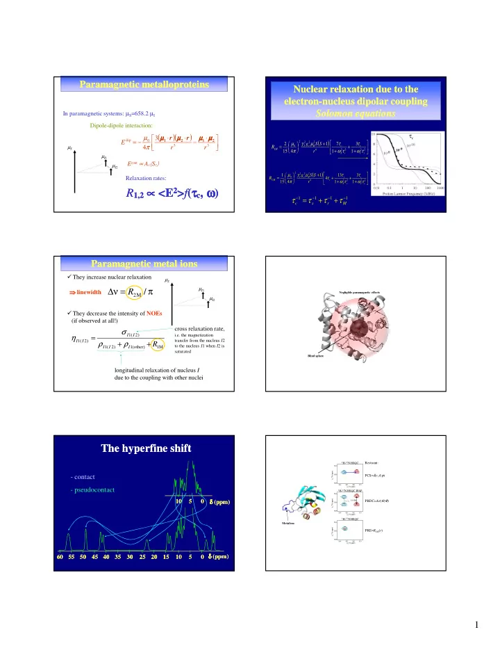
In paramagnetic systems: µS=658.2 µI Dipole-dipole interaction:

( )( )

• ⋅

− ⋅ ⋅ − =

3 5 dip

3 4 r r E

2 1 2 1

µ µ µ µ µ µ µ µ µ µ µ µ µ µ µ µ r r π µ

R1,2

1,2 ∝

∝ ∝ ∝ ∝ ∝ ∝ ∝ <E <E2>f(τ τ τ τ τ τ τ τc

c,

, ω ω ω ω ω ω ω ω)

µS µI1 µI2

Relaxation rates:

Paramagnetic metalloproteins Paramagnetic metalloproteins

Econt ∝ AcSz

( )

• +

+ + +

• =

2 2 2 2 6 2 2 2 2 1

1 3 1 7 1 4 15 2

c I c c S c B e I M

r S S g R τ ω τ τ ω τ µ γ π µ ( )

• +

+ + + +

• =

2 2 2 2 6 2 2 2 2 2

1 3 1 13 4 1 4 15 1

c I c c S c c B e I M

r S S g R τ ω τ τ ω τ τ µ γ π µ

Nuclear relaxation due to the Nuclear relaxation due to the electron electron-nucleus dipolar coupling nucleus dipolar coupling Solomon equations Solomon equations

τc

1 1 1 1 − − − −

+ + =

M r s c

τ τ τ τ

µS µI1 µI2

They increase nuclear relaxation They decrease the intensity of NOEs (if observed at all!)

π = ∆ν /

M 2

R

M 1 (other) 1 ) 2 ( 1 ) 2 ( 1 ) 2 ( 1

R

I I I I I I I

+ + = ρ ρ σ η

longitudinal relaxation of nucleus I due to the coupling with other nuclei

Paramagnetic metal ions Paramagnetic metal ions

• linewidth

cross relaxation rate,

i.e. the magnetization transfer from the nucleus I2 to the nucleus I1 when I2 is saturated

Negligible paramagnetic effects Blind sphere

δ δ δ δ δ δ δ δ (ppm) (ppm) 5 10 10

The hyperfine shift The hyperfine shift

δ δ δ δ δ δ δ δ (ppm) (ppm) 5 10 10 20 20 25 25 15 15 35 35 40 40 30 30 50 50 55 55 45 45 60 60

• contact
• pseudocontact

8.4 8.3 8.2 8.1 128 126 124 δ1(

15N) (ppm)

δ2(

1H) (ppm)

8.4 8.3 8.2 8.1 128 126 124 δ1(

15N) (ppm)

δ2(

1H) (ppm)

8.4 8.3 8.2 8.1 128 126 124 δ1(

15N) (ppm)

δ2(

1H) (ppm)

Metal ion

1H-15N HSQC 1H-15N HSQC IPAP 94 Hz 114 Hz 1H-15N HSQC

Restraint: PCS=δ(r,ϑ,ϕ) PRDC=∆ν(Θ,Φ) PRE=R1M(r)

SLIDE 2

2

B0

<µ>≠0 <µ>=0

S

• e

Bg

µ − = I I

I

γ

• =

Magnetic moments and magnetic fields Magnetic moments and magnetic fields

=

B e

g µ

1.86 ×10−23 JT−1

> < − >= <

z e B

S g µ µ

Average magnetic moment Average magnetic moment

S

• e

Bg

µ − =

N

γ

• N

g

1H

5.59 2.81 ×10−26 JT−1

2H

0.86 0.43

3H

5.96 2.99

13C

1.40 0.71

14N

0.40 0.20

15N −0.57 −0.28 31P

2.26 1.14 400 MHz 1H Larmor frequency

=

263 GHz of electron Larmor frequency

B B g E

N N N

γ µ

• =

= ∆ B g E

B eµ

= ∆

µ is 658 times larger than µI

I N B e N N B e B e S

g B g B g ω γ µ γ γ µ µ ω

• =

= = mS=±½

B g E

B eµ

= ∆

B0

Paramagnetic systems: χ = paramagnetic susceptibility per molecule, independent on B0 and positive P1/P0=exp(-∆E/kT)

Paramagnetic susceptibility Paramagnetic susceptibility

µ χ µ B >= <

z y x <µ µ µ µ> z x y mS=±½

B g E

B eµ

= ∆

B0 B0

mS = −1/2

If geµBB0MS << kT

) 1 ( 3 + − >= < S S kT B g S

B e z

µ

Curie law:

) 1 ( 3

2 2

+ = > < = S S kT g B

e B

µ µ µ µ χ ( ) ( )

• −

− > < >= <

S S S S

M S M S M S M S S z S z

kT E kT E M S S M S S

, , , ,

/ exp / exp , | | ,

Zeeman energy of the level if no contribution from the orbital magnetic moment

,

B M g E

S B e M S

S

µ =

> < − >= <

z e B

S g µ µ

Curie law Curie law

• B
• =

> <

B ⋅ =

Zeeman

E

1.86 ·10-23 ·20/2 <<1.38·10-23 ·298

In systems that are orbitally non-degenerate, the anisotropy can be represented by an anisotropy of the g-factor

( ) ( )

• −

− > + < − >= < − >= <

i kk i i kk i i kk e kk i B kk kk B kk

kT E kT E S g L S g / 1 / 1 | | φ φ µ µ µ

S kk kk e kk

M g S g L >= + < φ φ | | Ei kk =

B M g

S B kk µ

Zeeman energy

kT S S gkk

B kk

3 ) 1 (

2 2

+ = µ µ χ

Valid with only one thermally populated multiplet of spin number S NO zero field splitting

Magnetic susceptibility anisotropy Magnetic susceptibility anisotropy

Bz Bx B0 <µ>x <µ>z <µ µ µ µ> If the orbital magnetic moment is considered, χ χ χ χ is anisotropic

µ B

• ⋅

= > < χ χ χ χ

<µ µ µ µ> is NOT PARALLEL to B0 <µ> is orientation dependent

Average magnetic moment Average magnetic moment

SLIDE 3

3

( ) ( )

• −

−

• −

> + < − > + < =

≠ i i i i i j j i j kk e kk i i kk e kk i B kk

kT E kT E E E S g L kT S g L / exp / exp | | 2 | |

2 2 2

φ φ φ φ µ µ χ

if the total energy of the system E0 >> Zeeman energy Energies of ground and excited states

Van Vleck equation Van Vleck equation

E0 = zero field splitting and ligand field energy

χ µ >∝ >∝< <

z

S

are anisotropic

The origin of contact shifts The origin of contact shifts

Contact shift

• ntact shift : c

: contribution to the

• ntribution to the

chemical shift due to the unpaired chemical shift due to the unpaired electron spin electron spin density density on the resonating

• n the resonating

nucleus nucleus

A: contact hyperfine contact hyperfine c coupling proportional to the spin

• upling proportional to the spin

density of the resonating nucleus density of the resonating nucleus The coupling constant between nucleus and e- I1…e- is called A the interaction is expressed by

S I⋅ = A H

Contact shifts Contact shifts

kT B S S g S

e B z

3 ) 1 ( + − >= < µ S I⋅ = A H

Kurland and McGarvey (1970) predict that <Si> and hence contact shift may be orientation dependent due to spin-orbit coupling

H.M. McConnell, D.B. Chesnut, J.Chem.Phys. 1958, 28, 107-117

R.J. Kurland, B.R. McGarvey, J.Magn.Reson. 1970, 2, 286-301

C2 dxy dxz dyz

Electronic configuration of Electronic configuration of LS Fe LS FeIII

III Heme

Heme

I II III IV x y θ

3

1 3 5 8

φ φ φ φ

• φ

φ φ φ π π π π

g xx

Fe C N N N N N N N

( ) ( )

1 . 6 cos 8 . sin 4 . 18

2 2

+ + − − = φ θ φ θ δ

i i i

Calculated vs. observed shifts of methyl Calculated vs. observed shifts of methyl protons in histidine protons in histidine-cyanide cytochromes cyanide cytochromes

• I. Bertini, C. Luchinat, G. Parigi, F.A. Walker, JBIC 1999

I II III IV x y θ

3 1 3 5 8

φ φ φ φ

• φ

φ φ φ π π π π

g xx

N N Fe N

Contact shift restraints: Contact shift restraints: unpaired electron spin density unpaired electron spin density

• n heme nuclei is a function of axial ligand orientation
• n heme nuclei is a function of axial ligand orientation

8-CH3 5-CH3 1-CH3 3-CH3

M80A cyano-cytochrome c

Methyl protons in histidine cytochromes (Low spin Fe(III)) Low spin Fe(III))

From the fit of the methyl shifts: φ = 57o ± 9o

• structure

49 = φ

Banci, Bertini at al. JBIC (1996) Bren, Gray, Banci, Bertini, Turano J.Am.Chem.Soc. (1995)

SLIDE 4

4

Contact shift restraints: iron Contact shift restraints: iron-sulfur proteins sulfur proteins

kT S S g A S B A

N B c z I c con

γ µ γ ν ν ∆ 3 ) 1 (

2 2

+

• =

> <

• −

=

• Hβ

β β β β β β β of iron

• f iron-coordinated cysteines

coordinated cysteines

Bertini, Capozzi, Luchinat, Piccioli, Vila, Bertini, Capozzi, Luchinat, Piccioli, Vila,

• J. Am. Chem. Soc.,
• J. Am. Chem. Soc., 1994

1994

Fe Fe e- H S C θ θ θ θ θ θ θ θ δ δ δ δ δ δ δ δ ∝ ∝ ∝ ∝ ∝ ∝ ∝ ∝ sin sin2

2 θ

θ θ θ θ θ θ θ θ θ θ θ θ θ θ θ = M = M-S-C-H

B0 µ µ µ µ1 µ µ µ µ2 r

( )( )

• ⋅

− ⋅ ⋅ − =

3 5

3 4 r r H

2 1 2 1

• r
• r
• π

µ I I

I

γ

• =

( )( )

B

• I

B

• I

B

• r

r I ⋅ ⋅ =

• ⋅

⋅ − ⋅ ⋅ ⋅ − =

I I

r r H γ π γ

• 3

5

3 4 µ B

• ⋅

= > < χ χ χ χ

Electron Electron-nucleus dipole nucleus dipole-dipole interaction dipole interaction

Dipolar shift tensor

• −

− − − =

zz yy xx zz yy xx zz yy xx

r z yz xz yz r y xy xz xy r x r χ χ χ χ χ χ χ χ χ π σ ) 3 ( 3 3 3 ) 3 ( 3 3 3 ) 3 ( 4 1

2 2 2 2 2 2 5

The rotational average of the dipolar interaction causes a shift

• f the NMR signals, called pseudocontact shift:

δpcs = <Dipolar energy> / Zeeman energy ( )

B I

I z γ

• Pseudocontact shifts

Pseudocontact shifts

) ( 3 1

pcs

σ δ Tr − =

Note: if χ is isotropic, δpcs = 0 in the principal frame of the χ χ χ χ tensor

2 2 2 2 2 2 2 3 pcs

) 3 ( ) 3 ( ) 3 ( 12 1 r r z r y r x r

zz yy xx

χ χ χ π δ − + − + − =

( )

• +

− = ϕ ϑ χ ∆ ϑ χ ∆ π δ 2 cos sin 2 3 1 cos 3 12 1

2 2 3 pcs rh ax

r

. 2

rh ax yy xx yy xx zz

χ χ χ χ χ χ χ − = ∆ + − = ∆

Pseudocontact shifts Pseudocontact shifts

In polar coordinates: written in the frame of the χ tensor

z y x ϕ

ϑ r

M

• −

− − + → 

• iso

zz iso yy iso xx iso zz yy xx

I χ χ χ χ χ χ χ χ χ χ

Axial Totally Rhombic positive negative

Pseudocontact shifts Pseudocontact shifts

Surfaces with constant δpcs values:

rh =

∆χ

ax rh

) 3 / 2 ( χ χ ∆ = ∆

• proportional to r−

− − −3

the effect is propagated to atoms far from the paramagnetic center (R1 propagates as r−6)

• depend on angular parameters

provide information on the spatial position of the atom with respect to the metal ion Problems: *strong covariance between θ, φ and r *angular dependence provided by quadratic trigonometric functions: they are difficult to be used efficiently as retraints in torsion angle dynamics programs like DYANA/CYANA or Xplor-NIH

Pseudocontact shifts Pseudocontact shifts

( )

• +

− = ϕ ϑ χ ∆ ϑ χ ∆ π δ 2 cos sin 2 3 1 cos 3 12 1

2 2 3 pcs rh ax

r

SLIDE 5

5

Dipolar interaction between nuclear magnetic moments:

( )

1 cos 3 4

2 3 2

− − = γ γ γ π µ

B z A z AB B A

I I r H

• )

(cos d ) 1 cos 3 ( 2 1

1 1 2

= −

• −

γ γ Rotational average:

> − < − = ∆ = ∆ 2 1 cos 3 4

2 3 2 rdc

γ π γ γ µ ν

AB B A

r h E

• different orientations not all equally populated

( ) ( ) [ ]

Φ Θ − + − Θ − = ∆ 2 cos sin 1 cos 3 8

2 2 3 2 rdc yy xx zz AB B A

S S S r π γ γ µ ν

• A

B B

1 2

µ µ µ µ µ µ µ µ γ r ( )( )

• ⋅

− ⋅ ⋅ − =

3 5

3 4 r r H

2 1 2 1

• r
• r
• π

µ

Residual dipolar couplings Residual dipolar couplings

Orientation tensor bilayer micelle bicelle

Partial orientation Partial orientation

Orientation induced by restriction in space B0

( ) ( )

• +

− − = φ θ θ π γ γ π µ 2 cos sin 2 3 1 cos 3 2 4 ) (

2 2 3 2 rh ax AB B A

D D r h Hz rdc

Self Self-orientation rdc

• rientation rdc

The nuclear spin – nuclear spin interaction energy averages zero upon rotation Consequences: The molecular orientations are not equally probable The N-H dipole-dipole interaction does not average zero upon rotation ( )

sin ) 1 cos 3 (

2 2 1

≠ − ∝

π

γ γ γ γ µ d E

Anisotropic electron average magnetic moment µ µ µ µ µ µ µ µs

r

τ

r

τ µ µ µ µ µ µ µ µs

s

B0 Advantages of paramagnetic rdc

No perturbations due to the interactions with the

• rienting material

Disadvantages of paramagnetic rdc Line broadening due to the presence of the paramagnetic

• ion. However, line broadening is ∝ r-6

no disadvantages far from the paramagnetic ion Common disadvantages Simulated annealing protocols not optimized for multiple minima constraints

Self orientation versus orientation Self orientation versus orientation induced by external agents induced by external agents

aniso

2µ

µ

B

• B
• d

B ⋅ ⋅ − = > < ⋅ − =

> <

E

In paramagnetic systems:

• −

− − = β α β α β α β α α d d kT E d d kT E Sii cos ) / ) , ( exp( cos ) / ) , ( exp( 2 1 cos 3

aniso aniso 2

The orientation tensor S:

( )

χ χ µ − =

ii ii

kT B S

2

15 2 3

Self Self-orientation tensor

• rientation tensor

The magnetic susceptibility anisotropy induces molecular orientation ∝ ∝ ∝ ∝ B0. The rdc interaction is dependent on the

• rientation of NH vectors with respect

to the main axes of the χ χ χ χ tensor

• !"# !"$

%&&&'(# !!)$ '*+,-%.# !!/$ χ χ χ χxx χ χ χ χyy χ χ χ χzz

Bo

• ϕ

ϕ ϕ ϕ ϕ ϕ ϕ ϕ θ θ θ θ θ θ θ θ

15 15N 1H

( ) ( )

• ∆

+ − ∆ − = φ θ χ θ χ π γ γ π 2 cos 2 3 1 cos 3 4 15 4 1 ) (

2 2 3 2 2

sin r h kT B Hz rdc

mol rh mol ax HN N H

Self Self-orientation rdc

• rientation rdc

SLIDE 6

6

• depend on the NH / CαHα / C’Cα / … vector orientation
• do not depend on any distance with respect to the metal ion

Therefore, values of the same order of magnitude can be obtained for all the coupled nuclei of the protein

• they all refer to the same reference system, and thus relate all

the internuclear vectors to the same frame (and not the internuclear vectors to one another).

Residual dipolar couplings Residual dipolar couplings

( ) ( )

• ∆

+ − ∆ − = φ θ χ θ χ π γ γ π 2 cos 2 3 1 cos 3 4 15 4 1 ) (

2 2 3 2 2

sin r h kT B Hz rdc

mol rh mol ax HN N H

( )

• ∆

+ − ∆ = φ θ χ θ χ π δ 2 cos sin 2 3 1 cos 3 12 1

2 2 3 rh ax pc

r

( ) ( )

• +

− − = Φ Θ χ ∆ Θ χ ∆ π γ γ π ν ∆ 2 cos sin 2 3 1 cos 3 4 15 4 1 ) (

2 2 3 2 2 mol rh mol ax HN N H

r h kT B Hz

Pseudocontact shift Residual Dipolar Coupling

r, θ and φ are the polar coordinates of the resonating nucleus in the metal χ frame Θ and Φ are the angles defining the orientation of the NH vector in the molecular χ frame z y x ϕ

ϑ r

M z y x Φ

Θ rAB

A B M

Pseudocontact Shifts Residual Dipolar Couplings

∆νmol − ∆νdia = ∆νrdc

para

( ) ( )

• ∆

+ − ∆ − = ∆ φ θ χ θ χ π γ γ π 2 cos sin 2 3 1 cos 3 4 15 4 1 ) (

2 2 3 2 2 para rh para ax HN N H

r h kT B Hz rdc

∆χpara shiftpara − shiftdia = pcs

RDC obtained by difference between splittings measured on the paramagnetic and the diamagnetic sample at the same field depend on ∆χpara

PCS + RDC PCS + RDC

para RDC dia RDC 1 1

) ( ν ν ∆ + ∆ + = J B J

Three atoms, the same metal ion Three metal ions, the same atom

Pseudocontact shifts Pseudocontact shifts

Three NH, the same metal ion Two metal ions, the same NH

Residual dipolar couplings Residual dipolar couplings

SLIDE 7

7 Pseudocontact shifts in cytochrome b Pseudocontact shifts in cytochrome b5

Porphyrin containing a LS Fe(III) ion

Positive PCS Negative PCS calbindin D9k

Ce(III) Yb(III) Dy(III)

Too broad lines Too small PCS Different Lanthanides are substituted in the same binding site

Refining different shells around the metal Refining different shells around the metal

Positive pcs Negative pcs

• Φ

Θ ∆ + − Θ ∆ − = ∆ 2 cos sin 2 3 ) 1 cos 3 ( 2 15 4 1

2 2 3 2 rh ax AB B A para RDC

r kT B χ χ π γ γ π ν

• Ce(III)

calbindin D9k NH-N RDC in Ce(III)Calbindin D

N RDC in Ce(III)Calbindin D9k

9k ( ) ( ) ( )

• −

+ −

• +

− = φ θ χ χ θ χ χ χ π δ 2 cos sin 2 3 1 cos 3 2 1 12 1

2 2 3 yy xx yy xx zz i pc

r

• 1. Given ri, θ, φ and ∆χ’s, it is straightforward to find δpc
• 2. Given ri, θ and φ and δpc, it is still straightforward to

find ∆χ’s

• 3. Given δpc only, there is not a univocal set of the other

parameters

Considerations on the functional form of PCS Considerations on the functional form of PCS

• 1. Given θ, φ and ∆χ’s, it is straightforward to find

∆νRDC

• 2. Given θ, φ and ∆νRDC, it is still straightforward

to find ∆χ’s

• 3. Given ∆νRDC only, there is not a univocal set of

the other parameters ( ) ( )

• ∆

+ − ∆ − = ∆ φ θ χ θ χ π γ γ π ν 2 cos sin 2 3 1 cos 3 4 15 4 1 ) (

2 2 3 2 2 rh ax HN N H RDC

r h kT B Hz

Considerations on the functional form of RDC Considerations on the functional form of RDC

Nuclear relaxation Nuclear relaxation by electron spins by electron spins

z y y x x Sz y y x x z y x z B0

• Pictorial decomposition of the electron spin magnetic moment

Decomposition of the electron-nucleus dipolar interaction

1 1 1 1 − − − −

+ + =

M r s c

τ τ τ τ Dipole-dipole interaction

1 1 1 − − −

+ =

M r Curie

τ τ τ Curie interaction

Sz

( )

• +

+ + +

• =

2 2 2 2 6 2 2 2 2 1

1 3 1 7 1 4 15 2

c I c c S c B e I M

r S S g R τ ω τ τ ω τ µ γ π µ

2 2 6 2 2 2 4 4 2 2

1 3 ) 3 ( ) 1 ( 4 5 2

Curie I Curie B e I

r kT S S g τ ω τ µ ω π µ + +

• +

( )

• +

+ + + +

• =

2 2 2 2 6 2 2 2 2 2

1 3 1 13 4 1 4 15 1

c I c c S c c B e I M

r S S g R τ ω τ τ ω τ τ µ γ π µ

• +

+ +

• +

2 2 6 2 2 2 4 4 2 2

1 3 4 ) 3 ( ) 1 ( 4 5 1

Curie I Curie Curie B e I

r kT S S g τ ω τ τ µ ω π µ

Solomon Curie

SLIDE 8

8

r = 10 Å 900 MHz τR = 10-8 s

τc

• 1 = τR
• 1

+ τs

• 1

10 50 1600 800 400 200 100 25

1H Line broadening in Hz

3200 2

Dipolar line broadening by different electron Dipolar line broadening by different electron magnetic moments and relaxation times magnetic moments and relaxation times

10 50

LS Fe(III)

1600 800 400 200 100 25 r = 10 Å 900 MHz τR = 10-8 s τc-1 = τR-1 + τs-1 3200 2

Ce(III) Yb(III) Tm(III) Tb(III) Dy(III) type I Cu(II) type II Cu(II)

1H Line broadening in Hz

HS Fe(III)

Dipolar line broadening by different electron Dipolar line broadening by different electron magnetic moments and relaxation times magnetic moments and relaxation times

S=1/2, R=e=2 ns, 700 MHz

6 2

r R

I

γ ∝

Copper(II): 3d9 In non-idealized geometry, the non-degenerate ground state is well separated from the first excited state.

• electron relaxation mechanisms are relatively inefficient:

long electron relaxation time (of the order of 10-9 s)

• g-anisotropy is small

Conf. ml of

• ccupied
• rbitals

L S Free ion conf. Ligand field

• ctahedral

(Oh) tetrahedral (Td ) square planar (D4h) square pyramid. (C4v) trigonal bipyram. (D3h) d9 2,2,1,1,0,0,

• 1,-1,-2

2 1/2

2D 2E 2T

• 2A
• 2A
• 2A

Ground state: 2S+1X, where X=S, P, D, F depending on the L value equal to 0, 1, 2, 3, respectively (A symmetry: non-degenerate ground state ) (E symmetry: doubly degenerate ground states ) (T symmetry: three possible ground states ) ∆χ ≈0.6⋅10-32 m3

Not observed due to dynamic Jahn-Teller distance (Å)

5 10 15 20 25 30

pcs (ppm) / rdc (Hz)

0.1 1 10 10 Hz 20 50 100 200 500 1000

S=1/2 ∆χax=0.6×10−32m3 τs=3000 ps

900 MHz

Copper(II) Copper(II)

“Paramagnetic” Linewidth (absolute maximal values) High spin iron(III): 3d5 due to the non-degenerate ground state

• electron relaxation mechanisms are relatively inefficient:

T1e of the order of 10-9 s

• Spin orbit coupling introduces a relatively small ZFS, which

modulation causes electron relaxation: T1e can be of 10-11 s (with D of the order of 10 cm-1) (A symmetry: non-degenerate ground state ) (E symmetry: doubly degenerate ground states ) (T symmetry: three possible ground states ) ∆χ ≈3⋅10-32 m3

?

Conf. ml of

• ccupied
• rbitals

L S Free ion conf. Ligand field

• ctahedral

(Oh) tetrahedral (Td ) square planar (D4h) square pyramid. (C4v) trigonal bipyram. (D3h) d5 2,1,0,-1,-2 0 5/2

6S 6A 6A

• 6A
• 6A
• 6A

Ground state: 2S+1X, where X=S, P, D, F depending on the L value equal to 0, 1, 2, 3, respectively

ZFS: mS=±5/2

• mS=±3/2
• mS=±1/2

∆χ ≈0.6⋅10-32 m3

SLIDE 9

9

distance (Å)

5 10 15 20 25 30

pcs (ppm) / rdc (Hz)

0.1 1 10 10 Hz 20 50 100 200 500 1000

S=5/2 ∆χax=3×10−32 m3 τs=100 ps

900 MHz

High Spin Fe(III) High Spin Fe(III)

“Paramagnetic” Linewidth (absolute maximal values)

(if large ZFS is present)

Ground state: 2S+1X, where X=S, P, D, F depending on the L value equal to 0, 1, 2, 3, respectively (A symmetry: non-degenerate ground state ) (E symmetry: doubly degenerate ground states ) (T symmetry: three possible ground states ) Low spin iron(III): 3d5 In non-idealized geometry, there are low-lying excited states

• electron relaxation mechanisms (Orbach) are very efficient:

short electron relaxation time (10-13 - 10-12 s)

• ∆χ ≈2.4⋅10-32 m3

Conf. ml of

• ccupied
• rbitals

L S Free ion conf. Ligand field

• ctahedral

(Oh) tetrahedral (Td ) square planar (D4h) square pyramid. (C4v) trigonal bipyram. (D3h) d5 2,1,0,-1,-2 0 1/2

6S

− −

2T

− −

2T

− −

• 2A

− −

• 2E

− −

2E (strong ligands)

distance (Å)

5 10 15 20 25 30

pcs (ppm) / rdc (Hz)

0.1 1 10 10 Hz 20 50 100 200 500 1000

S=1/2 ∆χax=2.4×10−32m3 τs=1 ps

900 MHz

(absolute maximal values)

Low Spin Fe(III) Low Spin Fe(III)

“Paramagnetic” Linewidth Limit for signal detectability and assignment with standard experiments Blind zone

Max |RDC| Max |PCS|

limit for pcs detectability Ground state: 2S+1X, where X=S, P, D, F depending on the L value equal to 0, 1, 2, 3, respectively (A symmetry: non-degenerate ground state ) (E symmetry: doubly degenerate ground states ) (T symmetry: three possible ground states ) High spin iron(II): 3d6 In non-idealized geometry, there are low-lying excited states

• electron relaxation mechanisms (Orbach) are very efficient:

short electron relaxation time (10-12 s)

• ∆χ ≈2.1⋅10-32 m3

Conf. ml of

• ccupied
• rbitals

L S Free ion conf. Ligand field

• ctahedral

(Oh) tetrahedral (Td ) square planar (D4h) square pyramid. (C4v) trigonal bipyram. (D3h) d6 2,2,1,0,-1,

• 2

2 2

5D 5T 5E

• 5E
• 5A
• 5E

distance (Å)

5 10 15 20 25 30

pcs (ppm) / rdc (Hz)

0.1 1 10 10 Hz 20 50 100 200 500 1000

S=2 ∆χax=2.1×10−32m3 τs=1 ps

900 MHz

High Spin Fe(II) High Spin Fe(II)

(absolute maximal values) “Paramagnetic” Linewidth Ground state: 2S+1X, where X=S, P, D, F depending on the L value equal to 0, 1, 2, 3, respectively (A symmetry: non-degenerate ground state ) (E symmetry: doubly degenerate ground states ) (T symmetry: three possible ground states ) ∆χ ≈3⋅10-32 m3 High spin Cobalt(II): 3d7 In non-idealized geometry, there are low-lying excited states

• Distorted Octahedral (4T): very efficient electron relaxation

mechanisms: short electron relaxation time (10-12 s)

• Tetrahedral, D4h and D3h (4A): larger separation in energy

between the ground and the excited states, small ZFS: longer electron relaxation time (10-11 s)

• C4v (4E): intermediate because the low-lying excited states are relatively far.

Conf. ml of

• ccupied
• rbitals

L S Free ion conf. Ligand field

• ctahedral

(Oh) tetrahedral (Td ) square planar (D4h) square pyramid. (C4v) trigonal bipyram. (D3h) d7 2,2,1,1,0,- 1,-2 3 3/2

4F 4T 4A

• 4A
• 4E
• 4A

∆χ ≈7⋅10-32 m3

SLIDE 10

10

distance (Å)

5 10 15 20 25 30

pcs (ppm) / rdc (Hz)

0.1 1 10 10 Hz 20 50 100 200 500 1000

S=3/2 ∆χax=5×10−32 m3 τs=10 ps

900 MHz

Cobalt(II) Cobalt(II)

“Paramagnetic” Linewidth (absolute maximal values) Ground state: 2S+1X, where X=S, P, D, F depending on the L value equal to 0, 1, 2, 3, respectively (A symmetry: non-degenerate ground state ) (E symmetry: doubly degenerate ground states ) (T symmetry: three possible ground states ) Manganese(II): 3d5 (like high spin iron(III) ) due to the non-degenerate ground state electron relaxation mechanisms are relatively inefficient. Spin orbit coupling introduces a relatively small ZFS, generally smaller than that in high spin iron(III) - because the spin orbit coupling constant is smaller due to the smaller charge of the manganese(II) ion, and because excited states are closer in manganese(II) than in iron(III) -: T1e of the order of 10-9 -10-10 s (D around 1 cm-1)

Conf. ml of

• ccupied
• rbitals

L S Free ion conf. Ligand field

• ctahedral

(Oh) tetrahedral (Td ) square planar (D4h) square pyramid. (C4v) trigonal bipyram. (D3h) d5 2,1,0,-1,-2 0 5/2

6S 6A 6A

• 6A
• 6A
• 6A

Ground state: 2S+1X, where X=S, P, D, F depending on the L value equal to 0, 1, 2, 3, respectively ∆χ ≈0.2⋅10-32 m3 Gadolinium(III): 4f7 Non degenerate ground state; modulation of the transient ZFS is the dominant electron relaxation mechanism: T1e ≥ 2×10-10 s

Conf. ml of occupied orbitals L S Free ion conf. f7 3,2,1,0,-1,-1,-2,-3 7/2

8S

distance (Å)

5 10 15 20 25 30

pcs (ppm) / rdc (Hz)

0.1 1 10 10 Hz 20 50 100 200 500 1000

S=7/2 ∆χax=0.2×10−32m3 τs=10000 ps

900 MHz

Gadolinium(III) Gadolinium(III)

“Paramagnetic” Linewidth (absolute maximal values) Ground state: 2S+1X, where X=S, P, D, F,… depending on the L value equal to 0, 1, 2, 3, … ∆χ ≈2-40⋅10-32 m3 Lanthanide ions, with the exception of gadolinium(III) and europium(II), have low-lying excited states, due to strong spin-orbit coupling. Electron relaxation likely due to Orbach, with T1e< 10-12 s.

Ion

Configuration

2S+1LJ of ground

state (multiplicity in parentheses) gJ Ce3+ 4f1

2F5/2 (6)

6/7 Pr3+ 4f2

3H4 (9)

4/5 Nd3+ 4f3

4I9/2 (10)

8/11 Pm3+ 4f4

5I4 (9)

3/5 Sm3+ 4f5

6H5/2 (6)

2/7 Gd3+ 4f7

8S7/2 (8)

2 Tb3+ 4f8

7F 6 (13)

3/2 Dy3+ 4f9

6H15/2 (16)

4/3 Ho3+ 4f10

5I8 (17)

5/4 Er3+ 4f11

4I15/2 (16)

6/5 Tm3+ 4f12

3H6 (13)

7/6 Yb3+ 4f13

2F7/2 (8)

8/7 ) 1 ( 2 ) 1 ( ) 1 ( ) 1 ( 1 + + + + − + + = J J S S L L J J g J

distance (Å)

5 10 15 20 25 30

pcs (ppm) / rdc (Hz)

0.1 1 10 10 Hz 20 50 100 200 500 1000

J=5/2 ∆χax=2×10−32 m3 τs=0.1 ps

900 MHz

Cerium(III) Cerium(III)

“Paramagnetic” Linewidth (absolute maximal values)

SLIDE 11

11

distance (Å)

5 10 15 20 25 30

pcs (ppm) / rdc (Hz)

0.1 1 10 10 Hz 20 50 100 200 500 1000

J=7/2 ∆χax=7×10−32 m3 τs=0.3 ps

900 MHz

Ytterbium(III) Ytterbium(III)

“Paramagnetic” Linewidth (absolute maximal values)

distance (Å)

10 20 30 40

pcs (ppm) / rdc (Hz)

0.1 1 10 10 Hz 20 50 100 200 500 1000

J=6 ∆χax=20×10−32 m3 τs=0.5 ps

900 MHz

Thulium Thulium(III) (III)

“Paramagnetic” Linewidth (absolute maximal values)

distance (Å)

10 20 30 40

pcs (ppm) / rdc (Hz)

0.1 1 10 100 20 50 100 200 500 1000 10 Hz

J=6 ∆χax=35×10−32 m3 τs=0.3 ps

900 MHz

Terbium(III) Terbium(III)

“Paramagnetic” Linewidth (absolute maximal values)

distance (Å)

10 20 30 40

pcs (ppm) / rdc (Hz)

0.1 1 10 100 20 50 100 200 500 1000 10 Hz

900 MHz

J=15/2 ∆χax=35×10−32 m3 τs=0.5 ps

Dysprosium(III) Dysprosium(III)

“Paramagnetic” Linewidth (absolute maximal values)

Blind sphere Blind sphere Blind sphere

τe > 10 ns; ∆χ ≈ 0 (radicals) Metals with large ∆χ (Co2+, Tb3+, Tm3+, Dy3+...) Metals with large τe (<10 ns) (Cu2+, Mn2+, Gd3+...) PCS ≈ 0 PRE ≈ 0 PCS ≈ 0 R2 >> R1 Detectable PCS (R2

* < PCS)

Detectable PRE (R1 ≈ R2)

Structure calculations with Structure calculations with paramagnetism paramagnetism-based restraints based restraints

Classical + Paramagnetism-based (R1, CS, PCS, RDC…) restraints Metal ion and magnetic susceptibility tensor

The position of the metal can be determined without any assumption

Paramagnetic protein Paramagnetic protein Diamagnetic protein Diamagnetic protein

Classical restraints (NOE, dihedral angles, H-bonds…)

SLIDE 12

12

χ tensor components protein structure χ tensor components Protein coordinates PCS, RDC χold ≠ χnew PARAMAGNETIC CYANA NOEs, etc. END

NO YES

FANTASIAN, FANTAORIENT

Structure calculations with PCS and RDC Structure calculations with PCS and RDC

RDC PCS

ax

χ ∆

rh

χ ∆

Convergence of anisotropy parameters Convergence of anisotropy parameters

a protein containing LS Fe(III)

Banci, Bertini, Bren, Cremonini, Gray, Luchinat, Turano, JBIC 1, 117 (1996) δpcobs (ppm) δpcobs (ppm)

Solution structure of M80A cytochrome c Solution structure of M80A cytochrome c-

• CN

CN

Initial structural family Final structural family (NOE-only) (+ 280 pcs values) + 280 pcs values NOE-only

Banci, Bertini, Bren, Cremonini, Gray, Luchinat, Turano, JBIC 1, 117 (1996)

Solution structure of M80A cytochrome c Solution structure of M80A cytochrome c-CN CN

RDC, PCS, CCR, T1, CS and NOE are consistent with one another All constraints are included in PARAMAGNETIC DYANA# (CYANA#), and PARArestraints for Xplor-NIH* available at

www.cerm.unifi.it Building up an integrated package to Building up an integrated package to exploit paramagnetic constraints exploit paramagnetic constraints

#Güntert, Wütrich, J.Mol.Biol. 1991; Herrmann, Güntert, Wütrich, J.Mol.Biol. 2002 *Clore, Gronenborn, Brunger, Karplus, J.Mol.Biol. 1985; Schwieters, Kuszewski, Tjandra,

Clore, J.Magn.Reson., 2003

Solution structure calculation protocol Solution structure calculation protocol

• Least square penalty energy:

( ) [ ]

− − =

l i i calc i

• bs

i l

X X w E

2 , ,

, tol max

• Force constants wl do not change during the calculation
• Force constants wl were calibrated in such a way that each class of

restraints has a comparable contribution to the energy with respect to the standard restraints

• The contributions to the energy gradient from each class of

restraints are calculated as the first derivative of the energy terms, E, with respect to the coordinates

SLIDE 13

13

• 1793 NOEs
• 57 phi values
• 46 psi values
• 30 Hbonds
• 13 1D-NOE (RMSD=0.69Å)

Paramagnetic constraints: Paramagnetic constraints:

• 1164 pcs from 11 lanthanides
• 26 T1 values
• 254 rdc from 7 lanthanides
• 50 ccr from Ce(III) (RMSD=0.26 Å)

Diamagnetic constraints: Diamagnetic constraints:

Paramagnetism Paramagnetism-based restraints in based restraints in Calbindin D Calbindin D9k

9k

20 40 60 80 0.0 0.2 0.4 0.6 0.8 1.0 1.2 1.4 1.6 1.8 2.0 2.2 2.4 2.6

Paramagnetic structure Diamagnetic structure RMSD backbone Residue Number

Paramagnetism Paramagnetism-based restraints in based restraints in Calbindin D Calbindin D9k

9k

Towards structure Towards structures without NOEs without NOEs

50 100 150 200 250 1800 2000 1 2 3 4 5

BB RMSD (Å) number of NOEs

Bertini, Donaire, Jiménez, Luchinat, Parigi, Piccioli, Poggi, J. Biomol. NMR 2001

Structure can be

• btained with PCS,

RDC and less than 10 NOEs

+ 908 + 908 pcs pcs Ce, Yb, Dy +1703 Ce, Yb, Dy +1703 pcs pcs 11 lanthanides 11 lanthanides RMSD=1.28 Å RMSD=0.82 Å RMSD=1.28 Å RMSD=0.82 Å 17 hydrogen bonds, 105 dihedral angles, 17 hydrogen bonds, 105 dihedral angles, + 26 + 26 T1

1 Ce(III)

Ce(III) + 181 HN + 181 HN-

• N

N rdc rdc Ce(III), Dy(III) and Yb(III) Ce(III), Dy(III) and Yb(III)

Barbieri, Luchinat, Parigi, ChemPhysChem, 2004

Solid state NMR Solid state NMR CoMMP CoMMP-12 12 vs vs ZnMMP ZnMMP-12 12

PCS

13C-13C PDSD 11.5kHz MAS

ZnMMP-12 (Blue, Diamagnetic) CoMMP-12 (Red, Paramagnetic)

Balayssac, S.; Bertini, I.; Lelli, M.; Luchinat, C.; Maletta, M. J. Am. Chem. Soc. (2007), 129, 2218–2219

Solution Solution vs vs Solid Solid-State State PCS PCS

• 3
• 2
• 1

1 2 3 4 5 6 50 100 150 200 250 solid obs solid calc liquid obs liquid calc

PCS (ppm)

K151-A157 S230-A234 Balayssac, S.; Bertini, I.; Lelli, M.; Luchinat, C.; Maletta, M. J. Am. Chem. Soc. (2007), 129, 2218–2219

13C nuclei 13C 13C 13C 13C 13C 13C 13C 13C 13C 13C 13C 13C 13C 13C 13C

Me

+ = Intramolecular PCS Intermolecular PCS Total PCS

13C 12C 13C 12C 12C 12C 12C

Paramagnetic labeling scheme for the measurement of intramolecular PCS

13C 12C 12C 13C 12C 12C 12C

Paramagnetic labeling scheme for the measurement of intermolecular PCS

Diamagnetic Metal

SLIDE 14

14

CoMMP CoMMP-12 12 Pseudo Contact Shifts: Pseudo Contact Shifts: Intra Intra-

• and

and Inter Inter-Molecular Effects Molecular Effects

Intra-Molecular and Inter-Molecular PCS

Interaction with all the Co2+ lattice ions

29 Å 35 Å 24 Å 20 Å 9.4 Å A 9.6 Å B 40 Å 30 Å

x y z A

29 Å 35 Å 24 Å 20 Å 9.4 Å A 9.6 Å B 40 Å 30 Å

x y z x y z A

Ser 230

12.0 Å

Nearest Co2+ Atom Bound Co2+ Atom

10.5 Å

Balayssac, S.; Bertini, I.; Lelli, M.; Luchinat, C.; Maletta, M. J. Am. Chem. Soc. (2007), 129, 2218–2219

Co2+ ions

13C-15N

Co-MMP12

13C-15N

Zn-MMP12

Paramagnetic-diluted sample Reversed Paramagnetic-diluted

Inter PCS Intra PCS

Paramagnetic Paramagnetic-diluted samples: diluted samples: Direct and Direct and Reverse Dilution Reverse Dilution

Intra and intermolecular PCS can be separated

Balayssac, S.; Bertini, I.; Bhaumik, A.; Lelli, M.; Luchinat, C., PNAS, (2008), 105, 17284-17289

High Resolution Protein Structure with PCS

X X X X-

• ray

ray ray ray with PCS with PCS with PCS with PCS without PCS without PCS without PCS without PCS RMSD (Å) BB

1 1 1 1. . . .0

(1.3 Å to X-ray)

1 1 1 1. . . .3 3 3 3 (1.6 Å to X-ray)

Secondary elements (BB)

0. . . .9 9 9 9 (1.0 Å to X-ray) 1 1 1 1. . . .1 1 1 1(1.3 Å to X-ray)

Restraints Restraints Restraints Restraints DARR/PDSD 161 161 CHHC 221 221 PAR 297 297 PAIN 98 98 TALOS 186 186 Metal links 3 3 PCS 318

Bertini, I.; Bhaumik, A.; De Paëpe, G; Griffin, R.G.; Lelli, M.; Lewandowski, J.R.; Luchinat, C. J.Am.Chem.Soc., 2010, 132, 1032

Structure calculations with total PCS (without dilutions)

1 2 3 4 5 6 7 5 10 15 20

Target Function number of metal ions

TF min TF average best 20 structures

1) Structural calculations are performed with the available restraints with different numbers of metal ions and estimated ∆χ anisotropy values 2) The minimum number of metal ions (4) needed to best fit the PCS is found from the TF values 3) From the calculated structural model, new restraints can be found The fourth metal is not clustered Internal metal Internal metal Second metal Second metal Third metal Third metal

(thicker line is the crystal structure)

BB RMSD to the mean = 0.9 Å BB RMSD with the X-ray structure = 1.4 Å

Structure calculations with total PCS (without dilutions)

4) Best fit of PCS to the structure provides new ∆χ values; structural calculation is repeated; and so on till convergence 5) Calculations are performed with a modified version

• f PARAMAGNETIC-CYANA with a single metal

ion, and all cystallographic molecules positioned from the knowledge of the cell symmetry and

• parameters. The position and orientation of the

crystallographic origin is obtained in the minimization Metal tensor Crystallographic origin Neighboring molecules are positioned according to the provided symmetry

5 10 15 20

• 3.0x10
• 32
• 2.0x10
• 32
• 1.0x10
• 32

0.0 1.0x10

• 32

2.0x10

• 32

3.0x10

• 32

4.0x10

• 32

5.0x10

• 32

6.0x10

• 32

7.0x10

• 32

8.0x10

• 32

9.0x10

• 32

1.0x10

• 31

1.1x10

• 31

1.2x10

• 31

1.3x10

• 31

Magnetic anisotropy (m

3)

iteration

axial rhombic

Structure calculations with total PCS (without dilutions)

In the case of MMP-12, in orthorombic symmetry, 4 cases are possible 1) P2 1) P21

121 12 (the correct symmetry!)

2 (the correct symmetry!) BB RMSD to the mean = 0.9 Å BB RMSD with the X-ray structure = 1.2 Å Without clashes between neighboring molecules

(thicker line is the crystal structure) Position and

• rientation of

the origin

NMR and X-ray crystals are in agreement

Luchinat, Parigi, Ravera, Rinaldelli, JACS 2012

SLIDE 15

15

Structure calculations with total PCS (without dilutions)

2) Symmetry P2 2) Symmetry P212121

Neighboring molecules clash!

3) Symmetry P222 3) Symmetry P222 4) Symmetry P222 4) Symmetry P2221

1

BB RMSD to the mean = 0.9 Å BB RMSD with the X-ray structure = 1.6 Å The TF is larger than in the P21212 case Without clashes between neighboring molecules

(thicker line is the crystal structure)

Luchinat, Parigi, Ravera, Rinaldelli, JACS 2012

PCS and RDC relative to one metal can provide the relative position of the metal and the χ χ χ χ tensor axes with respect to any rigid domain but not the directions of the χ tensor axes.

PCS and RDC provide an unique solution if two (or more) sets, relative to two different metal ions, are used. PCS provide information on the distance; RDC are more sensitive to the

• rientation of rigid bodies far from the metal ion

M

Rigid domains, pcs and rdc Rigid domains, pcs and rdc

( )

• ∆

+ − ∆ = φ θ χ θ χ π δ 2 cos sin 2 3 1 cos 3 12 1

2 2 3 rh ax i pc

r

Bertini, Longinetti, Luchinat, Parigi, Sgheri, J.Biomol.NMR (2002)

( ) ( )

• ∆

+ − ∆ − = φ θ χ θ χ π γ γ π 2 cos sin 2 3 1 cos 3 4 15 4 1 ) (

2 2 3 2 2 rh ax AB B A

r h kT B Hz rdc +

• × 4

jth helix jth helix-tensor structure

( )

• ∆

+ − ∆ φ θ χ θ χ 2 cos sin 2 3 1 cos 3

2 2 rh ax

The relative position of the metal ion with respect to any rigid domain can be determined but NOT the directions of the χ χ χ χ tensor axes. RDC and PCS values are fit to obtain the metal tensor: 23 orientations: 4 have correct chirality

Rigid domains Rigid domains

Unknown: coordinates of the metal (3), tensor parameters (5) + +…+

• j = 1

j = 2 j = n j = n j = 2 j = 1

× 4n−1

PCS and RDC do not provide a unique solution, unless two sets, relative to two different metal ions, are used.

Rigid domains Rigid domains

With two metals degeneracy is removed!

x y z x y z x y z x y z x y z x y z x y z x y z x y z x y z x y z x y z x y z x y z y x z x y z x y z x y z

Metal 1 Metal 2

• r

ith

• r

ith

From the position of the metal ion and the directions of χ χ χ χ tensor axes, all rigid domains can be relatively oriented

A possible strategy for structure calculation in solution: use the X-ray structure of individual “relatively rigid” domains to obtain the structure of the whole system from PCS and RDC.

Paramagnetic ions must be attached to one protein domain

M

Rigid domains, pcs and rdc Rigid domains, pcs and rdc

SLIDE 16

16

Cytochrome b562

Bertini, Longinetti, Luchinat, Parigi, Sgheri, J. Biomol. NMR 2002

Calbindin D9k

Attaching a paramagnetic ion Attaching a paramagnetic ion to the protein to the protein

Ln3+

N C

B0

Two approaches have been developed:

• paramagnetic binding tag with reduced flexibility
• substitution of a paramagnetic ion

in metalloproteins

Ln

N C

Tag B0

• 3
• 2
• 1

1 2 3 4

• 3
• 2
• 1

1 2 3 4 Tb Dy Tm

PCS obs (ppm) PCS calc (ppm)

PCS and RDC, plus crystal structure, are used to calculate the solution structure of complexes of CaM with target peptides from DAP (death-associated protein) kinases

Structural refinement in CaM complexes Structural refinement in CaM complexes

Calmodulin CaM-binding domain

X-ray structure

PCS provide the χ χ χ χ tensors

• 30
• 20
• 10

10 20 30

• 30
• 20
• 10

10 20 30

80 81 82 83 84 85 86 87 88 89 90 91 92 93 94 95 96 97 98 99 100 101 102 103 104 105 106 107 108 109 110 111 112 113 114 115 116 117 118 119 120 121 122 123 124 125 126 127 128 129 131 132 133 134 135 136 137 138 139 140 141 142 143 144 145 146 147 148 80 81 82 83 84 85 86 87 88 89 90 91 92 93 94 95 96 97 98 99 100 101 102 103 104 105 106 107 108 109 110 111 112 113 114 115 116 117 118 119 120 121 122 123 124 125 126 127 128 129 130 131 132 133 134 135 136 137 138 139 140 141 142 143 144 145 146 147 148 80 81 82 83 84 85 86 87 88 89 90 91 92 93 94 95 97 98 99 100 1 102 103 104 105 106 107 108 109 110 111 112 113 114 115 116 117 119 120 121 122 123 124 125 126 127 128 129 130 131 132 134 135 136 137 138 140 141 142 143 144 145 146 147 148

Tb Tm Dy

RDC obs (Hz) RDC C-ter calc (Hz)

• 30
• 20
• 10

10 20 30

• 30
• 20
• 10

10 20 30

3 4 5 6 7 8 9 10 11 12 13 14 15 16 17 18 19 20 37 38 39 40 41 42 44 45 46 47 50 76 77 78 79 3 4 5 6 7 8 9 10 11 12 13 14 15 16 17 18 19 20 21 22 23 24 31 32 33 34 35 36 37 38 39 40 41 42 44 45 46 47 48 49 72 73 74 3 4 5 6 7 8 9 10 11 12 13 14 15 16 18 37 38 40 41 42 44 45 46 47 50 77 78 79

Tb Tm Dy

RDC obs (Hz) RDC N-ter calc (Hz)

• Exp. RDC deviate from predictions based on the X-ray structure due to structural

rearrangements in solution

Structural refinement in CaM complexes Structural refinement in CaM complexes

RDC calculated from the X-ray structure and the χ tensor obtained from PCS are significantly different from experimental RDC

20 40 60 80 100 120 140 0.0 0.2 0.4 0.6 0.8 1.0 1.2 1.4 1.6

R1 (s

• 1)

Residue number

20 40 60 80 100 120 140 2 4 6 8 10 12 14 16 18

R2 (s

• 1)

Residue number

20 40 60 80 100 120 140 5 10 15 20

R2/R1 Residue number

Mobility measurements Mobility measurements

HYDRONMR predictions are shown as bars τ= 9.8 ns, in perfect agreement with HYDRONMR

Structural refinement in CaM complexes Structural refinement in CaM complexes

The protocol Xplor-NIH: simulated annealing at 200 K

Restraints: 1) φ and ψ angles extracted from the X-ray structure 2) PCS, to place the χ tensors 3) PCS+RDC+dihedral φ and ψ angles from TALOS Only PCS and RDC of residues not experiencing large mobility as revealed from relaxation measurements have been included

SLIDE 17

17

• 2

2 4

• 2

2 4 Tb Tm Yb PCS obs (ppm) PCS calc (ppm)

• 30
• 20
• 10

10 20 30

• 30
• 20
• 10

10 20 30 Tb Tm Yb RDC obs (Hz) RDC calc (Hz)

CaM solution structure in complex with CaM solution structure in complex with DAP kinase DAP kinase

Fit of PCS on the refined solution structure Fit of RDC of non-mobile atoms

• n the refined solution structure

X-ray structure ray structure NMR structure NMR structure

RMSD=2.0 Å

Chemical structure Chemical structure Experimental data Experimental data Prediction Prediction Model Model Forward problem Forward problem Inverse problem Inverse problem

A rigid two A rigid two-

• domain protein:

domain protein: a “well posed inverse problem” for NMR a “well posed inverse problem” for NMR

“Four “Four-dimensional” protein dimensional” protein structures structures

A1 B1 C D E A2 B2

Fragai, Luchinat, Parigi, Acc. Chem. Res., 2007

Our strategy Our strategy

A paramagnetic ion is included in the N-terminal domain PCS and RDC measured for atoms in the N-terminal domain are used to calculate the magnetic susceptibility anisotropy tensor PCS and RDC measured for atoms in the C-terminal domain provide information

• n the effects transmitted through the

linker, i.e. on the region of space sampled by the C-terminal

?

N-terminal

Ln3+

flexible linker C-terminal

The N60D mutant of calmodulin was used as it selectively binds lanthanides in the second binding loop of the N-terminal domain Bertini, Bertini, Del Bianco, Gelis, Katzaros, Del Bianco, Gelis, Katzaros, Luchinat, Parigi Luchinat, Parigi, , Peana, Provenzani, Zoroddu Peana, Provenzani, Zoroddu, , PNAS PNAS 2004, 101, 6841 2004, 101, 6841

RDC of N RDC of C RDC of C

Rigid system Mobile system

Differences in tensor magnitude between N Differences in tensor magnitude between N- and C and C-terminal will immediately point to terminal will immediately point to conformational freedom conformational freedom

If the adduct is not rigid, PCS and RDC of C-term are averaged over the values relative to all experienced conformations

Isotropic reorientation RDC = 0

N-terminal C-terminal Me N-terminal

• 30 -20 -10

10 20 30 Hz

• 30 -20 -10

10 20 30 Hz

• 30 -20 -10

10 20 30 Hz

RDC of N

C-terminal Me

• 30 -20 -10

10 20 30 Hz

Bertini, Bertini, Del Bianco, Gelis, Katzaros, Del Bianco, Gelis, Katzaros, Luchinat, Parigi Luchinat, Parigi, Peana, Provenzani, Zoroddu , Peana, Provenzani, Zoroddu, , PNAS, PNAS, 2004 2004 Bertini, Bertini, Gupta, Gupta, Luchinat, Parigi Luchinat, Parigi, Peana, Sgheri , Peana, Sgheri, Yuan , Yuan JACS, JACS, 2007 2007

Same tensors Same tensors Different tensors Different tensors

• 8
• 6
• 4
• 2

2 4 6

• 8
• 6
• 4
• 2

2 4 6 Observed values (ppm) Calculated values (ppm)

Tb3+ Tm3+ Dy3+ 37 26 34 ×10−32 m3

• 14 -9.1 -15 ×10−32 m3

ax

χ ∆

rh

χ ∆

Determining the Determining the χ χ χ χ χ χ χ χ tensors tensors

Tb3+/Tm3+/Dy3+ are substituted to Ca2+ in the second binding site of the N-terminal domain of N60D CaM PCS

N-domain

• 4
• 3
• 2
• 1

1 2 3 4

• 4
• 3
• 2
• 1

1 2 3 4 Calculated values (Hz) Observed values (Hz)

RDC

C-domain

Tb3+ Tm3+ Dy3+ −1.6 −3.3 −1.9 ×10−32 m3 0.8 2.2 0.8 ×10−32 m3

ax

χ ∆

rh

χ ∆

10-20 times smaller!

Bertini, Bertini, Gupta, Gupta, Luchinat, Parigi Luchinat, Parigi, Peana, Sgheri , Peana, Sgheri, Yuan , Yuan JACS, 2007 JACS, 2007

Averaged tensors

SLIDE 18

18

• 3 0
• 2 0
• 1 0

1 0 2 0 3 0

• 3 0
• 2 0
• 1 0

1 0 2 0 3 0

Tb3+ Tm3+ rdc of the N-terminal domain

RDC of N RDC of N- and C and C-terminal domains terminal domains

• 3 0
• 2 0
• 1 0

1 0 2 0 3 0

Dy3+

• 6
• 4
• 2

2 4 6

• 6
• 4
• 2

2 4 6

• 6
• 4
• 2

2 4 6

rdc of the C-terminal domain Tb3+ Tm3+ Dy3+ Ln3+

N C Distribution of the rdc values in the two domains

Ln3+

N C

Reduced rdc values implies MULTIPLE RECIPROCAL ORIENTATIONS

Chemical structures Chemical structures Experimental data Experimental data Prediction Prediction Model Model Forward problem Forward problem Inverse problem Inverse problem

?

A flexible two A flexible two-domain protein: domain protein: an ill an ill-posed inverse problem posed inverse problem

Wrong ensembles Wrong ensembles

Proteins move: Proteins move: The “four The “four-dimensional” dimensional” structure of proteins structure of proteins Fragai, Luchinat, Parigi, Fragai, Luchinat, Parigi,

• Acc. Chem. Res., 2007
• Acc. Chem. Res., 2007

PCS and RDC can be used together to obtain the maximum

• ccurrence (MO) for each conformation

Conformations with largest MO are those in which the system can stay longer

MO = maximum weight for a conformation independently of all

• ther experienced conformations

Maximum Occurrence calculation for the Maximum Occurrence calculation for the different conformations different conformations

Bertini, Gupta, Luchinat, Parigi, Peana, Sgheri, Yuan, JACS, 2007

Ln3+ Ln3+

Longinetti, Luchinat, Parigi, Sgheri, Inverse Problems, 2006 Bertini, Giachetti, Luchinat, Parigi, Petoukhov, Pierattelli, Ravera, Svergun, JACS, 2010

References:

• I. Bertini, C. Luchinat, G. Parigi, “Paramagnetic constraints: an aid for quick solution structure

determination of paramagnetic metalloproteins”, Concepts in Magn. Reson. (2002) 14, 259-286.

• I. Bertini, C. Luchinat, G. Parigi, “Magnetic susceptibility in paramagnetic NMR”, Progr. in NMR
• Spectr. (2002) 40, 249-273.
• I. Bertini, C. Luchinat, G. Parigi, “1H NMRD profiles of paramagnetic aquo-complexes and

metalloproteins”, Adv. Inorg. Chem. (2005) 57, 105-172. In R. van Eldik and I. Bertini, “Relaxometry of water-metal ion interactions”.

• I. Bertini, C. Luchinat, G. Parigi, R. Pierattelli, “NMR Spectroscopy of Paramagnetic

Metalloproteins”, ChemBioChem (2005) 6, 1536-1549.

• M. Fragai, C. Luchinat, G. Parigi, “Four dimensional protein structures: examples from

metalloproteins”, Acc. Chem. Res. (2006) 39, 909-917.

• I. Bertini, C. Luchinat, G. Parigi, R. Pierattelli, “Perspectives in paramagnetic NMR of

metalloproteins”, Dalton Trans. (2008) 3782-3790.

• I. Bertini, C. Luchinat, G. Parigi, “Moving the frontiers in solution and solid state bioNMR”,
• Coord. Chem. Rev. (2011) 255, 649-663.
• I. Bertini, C. Luchinat, G. Parigi, “Paramagnetic molecules” in “NMR of Biomolecules: Towards

Mechanistic Systems Biology”, Bertini I, McGreevy KS, Parigi G (Eds.), Wiley-VCH, Weinheim, Germany, 2012, pag. 155-171.

• M. Fragai, C. Luchinat, G. Parigi, E. Ravera, “Conformational freedom of metalloproteins revealed

by paramagnetism-assisted NMR”, Coord. Chem. Rev. (2013) 257, 2652-2667.

• A. Bhaumik, C. Luchinat, G. Parigi, E. Ravera, M. Rinaldelli, “NMR crystallography on

paramagnetic systems: solved and open issues”, CrystEngComm (2013) 15, 8639-8656.