Years of Life Lost to Diabetes Take, say 200, persons follow till - - PDF document

SLIDE 1

Years of Life Lost to Diabetes

Bendix Carstensen Steno Diabetes Center Gentofte, Denmark http://BendixCarstensen.com LEAD symposiun at EDEG, Dubrovnik, 6 May 2017 http://BendixCarstensen.com/Epi/Courses/EDEG2017

1/ 65

Expected Lifetime

Years of Life Lost to Diabetes LEAD symposiun at EDEG, Dubrovnik, 6 May 2017 http://BendixCarstensen.com/Epi/Courses/EDEG2017

Life lost to disease

◮ Persons with disease live shorter than persons without ◮ The difference is the life lost to disease — years of life lost ◮ Possibly depends on:

◮ sex ◮ age ◮ duration of disease ◮ definition of persons with/out disease

◮ Conditional or population averaged? ◮ . . . the latter gives a seductively comfortable single number ◮ . . . the former confusingly relevant insights ◮ YLL derives from Expected Lifetime

Expected Lifetime (erl-intro) 2/ 65

Expected Lifetime — the formals:

. . . the age at death integrated w.r.t. the distribution of age at death: EL = ∞ a f (a) da The relation between the density f and the survival function S is f (a) = −S ′(a), so integration by parts gives: EL = ∞ a

• −S ′(a)
• da = −
• aS(a)

∞

0 +

∞ S(a) da The first term is 0 so: EL = ∞ S(a) da — the area under the survival curve.

Expected Lifetime (erl-intro) 3/ 65

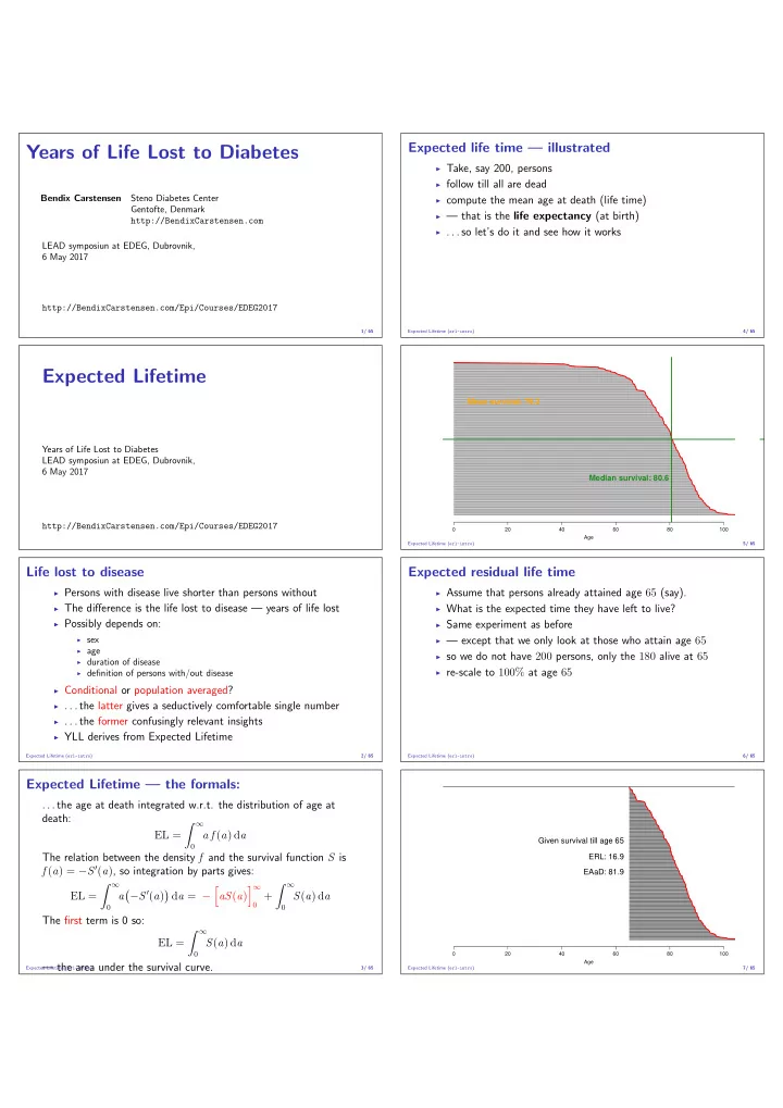
Expected life time — illustrated

◮ Take, say 200, persons ◮ follow till all are dead ◮ compute the mean age at death (life time) ◮ — that is the life expectancy (at birth) ◮ . . . so let’s do it and see how it works

Expected Lifetime (erl-intro) 4/ 65 20 40 60 80 100 Age

Median survival: 80.6 Mean survival: 79.2

Expected Lifetime (erl-intro) 5/ 65

Expected residual life time

◮ Assume that persons already attained age 65 (say). ◮ What is the expected time they have left to live? ◮ Same experiment as before ◮ — except that we only look at those who attain age 65 ◮ so we do not have 200 persons, only the 180 alive at 65 ◮ re-scale to 100% at age 65

Expected Lifetime (erl-intro) 6/ 65 20 40 60 80 100 Age

Given survival till age 65 ERL: 16.9 EAaD: 81.9

Expected Lifetime (erl-intro) 7/ 65

SLIDE 2

Expected lifetime and years lost

◮ ERL (Expected Residual Lifetime):

Area under the survival curve

◮ YLL (Years of Life Lost) (to diabetes, say):

ERLpop − ERLDM

◮ difference between areas under survival curve for persons

without DM and persons with DM

◮ ⇒ area between the survival curves ◮ . . . but not all use this approach

Expected Lifetime (erl-intro) 8/ 65

Years of Life Lost

Years of Life Lost to Diabetes LEAD symposiun at EDEG, Dubrovnik, 6 May 2017 http://BendixCarstensen.com/Epi/Courses/EDEG2017

Wikipedia: PYLL

Potential Years of Life Lost

◮ Fix a threshold, T, (the population EL, or say 75) ◮ A person dead in age a < T contributes T − a ◮ A person dead in age a > T contributes 0

. . . seems to assume that the expected age at death is T regardless

• f attained age ?

Years of Life Lost (yll-intro) 9/ 65

WHO — Years of Life Lost

Rationale for use Years of life are lost (YLL) take into account the age at which deaths occur by giving greater weight to deaths at younger age and lower weight to deaths at

• lder age. The years of life lost (percentage of total) indicator measures the YLL

due to a cause as a proportion of the total YLL lost in the population due to premature mortality. Definition YLL are calculated from the number of deaths multiplied by a standard life expectancy at the age at which death occurs. The standard life expectancy used for YLL at each age is the same for deaths in all regions of the world (. . . ) www.who.int/whosis/whostat2006YearsOfLifeLost.pdf

⇒ a person dying in age a contributes ERL(a) > 0

Years of Life Lost (yll-intro) 10/ 65

Comparing men and women

◮ When a man dies age a, say,

◮ YLL is ERLw(a)> 0 ◮ — the expected residual life time of a woman aged a.

◮ When a woman dies age a, say,

◮ YLL is ERLm(a)> 0 ◮ — the expected residual life time of a man aged a.

◮ . . . so each sex lose years relative to the other ! ◮ So maybe not a terribly useful measure.

Years of Life Lost (yll-intro) 11/ 65

The ad-hoc measures do not work

◮ anyone who dies before age 75 (PYLL) ◮ anyone who dies (WHO YLL) ◮ . . . contribute a positive number to YLL ◮ ⇒ any subgroup of the population have positive years of life

lost when compared to the general population!

◮ . . . actually, compared to any population (ex: men vs. women) ◮ They only use the dead persons and ignore the living ◮ No shortcuts:

◮ the YLL is a difference of expectations ◮ use a statistical model (specify f (a), that is) ◮ a statistical model for all persons ◮ We will use diabetes in Denmark as an example Years of Life Lost (yll-intro) 12/ 65

YLL — the details

Years of Life Lost to Diabetes LEAD symposiun at EDEG, Dubrovnik, 6 May 2017 http://BendixCarstensen.com/Epi/Courses/EDEG2017

How the world looks Well DM Dead Dead(DM) λ(a) µW(a) µDM(a,d) Well DM Dead Dead(DM)

YLL — the details (DK-ex) 13/ 65

SLIDE 3

Comparing DM and well

YLL = ∞ SW (a) − SD(a) da The survival functions we need are derived from mortality rates: SW (a) = exp

• −

a µW (u) du

• ,

SD(a) = exp

• −

a µD(u) du

• YLL — the details (DK-ex)

14/ 65

Mortality rates from Denmark

> library( Epi ) > clear() > data( DMepi ) > w15 <- subset( DMepi, sex=="F" & P==2015 ) > w15 <- w15[order(w15$A),] > w15 <- transform( w15, mW = D.nD / Y.nD, # no DM mortality + iW = X / Y.nD, # DM incidence + mD = pmax(0,D.DM / Y.DM,na.rm=TRUE), # DM mortality + mT = (D.nD+D.DM)/(Y.nD+Y.DM) ) # total mortality > Sw <- surv1( 1, w15$mW ) > Sd <- surv1( 1, w15$mD ) > cbind( Sw, Sd )[65:70,] age A0 age A0 65 64 0.9297246 64 0.7853495 66 65 0.9226514 65 0.7721934 67 66 0.9149180 66 0.7547042 68 67 0.9070037 67 0.7381123 69 68 0.8990846 68 0.7214464 70 69 0.8909150 69 0.7061645

YLL — the details (DK-ex) 15/ 65

Survival curves (?)

20 40 60 80 100 0.0 0.2 0.4 0.6 0.8 1.0 Age Survival

Well DM

YLL — the details (DK-ex) 16/ 65

Comparing DM and well

YLL = ∞ SW (a) − SD(a) da The survival functions we need are derived from mortality rates: SW (a) = exp

• −

a µW (u) du

• ,

SD(a) = exp

• −

a µD(u) du

• For the conditional YLL given attained age A, just use:

SW (a|A) = SW (a)/SW (A), SD(a|A) = SD(a)/SD(A)

YLL — the details (DK-ex) 17/ 65

Mortality rates from Denmark

> Sw <- surv1( 1, w15$mW, A=65 ) > Sd <- surv1( 1, w15$mD, A=65 ) > cbind( Sw, Sd )[65:70,] age A0 A65 age A0 A65 65 64 0.9297246 1.0000000 64 0.7853495 1.0000000 66 65 0.9226514 1.0000000 65 0.7721934 1.0000000 67 66 0.9149180 0.9916183 66 0.7547042 0.9773513 68 67 0.9070037 0.9830406 67 0.7381123 0.9558646 69 68 0.8990846 0.9744576 68 0.7214464 0.9342820 70 69 0.8909150 0.9656030 69 0.7061645 0.9144918

YLL — the details (DK-ex) 18/ 65

Conditional survival curves

20 40 60 80 100 0.0 0.2 0.4 0.6 0.8 1.0 Age Survival

Well DM

YLL — the details (DK-ex) 19/ 65

Comparing DM and well

YLL = ∞ SW (a) − SD(a) da The survival functions we need are derived from mortality rates: SW (a) = exp

• −

a µW (u) du

• ,

SD(a) = exp

• −

a µD(u) du

• For the conditional YLL given attained age A, just use:

SW (a|A) = SW (a)/SW (A), SD(a|A) = SD(a)/SD(A) This implicitly assumes that persons in“Well”cannot contract“DM” The immunity assumption — which is widely used in the literature

YLL — the details (DK-ex) 20/ 65

How the world looks

Well DM Dead Dead(DM) λ(a) µW(a) µDM(a) Well DM Dead Dead(DM) . . . with immunity to diabetes

YLL — the details (DK-ex) 21/ 65

SLIDE 4

Comparing DM and Well in the real world

YLL = ∞ SW (t) − SD(t) dt still the same, but SW (t) should be: SW (a) = P {Well}(a) + P {DM}(a)

Well DM Dead Dead(DM) λ(a) µW(a) µDM(a) Well DM Dead Dead(DM)

YLL — the details (DK-ex) 22/ 65

Comparing DM and well in the real world

The survival function SW (a) is the sum of: P {Well}(a) = exp

• −

a µW (u) + λ(u)

• du

and P {DM}(a) = a P {survive to s, DM diagnosed at s} × P {survive with DM from s to a} ds = a λ(s) exp

• −

s µW (u) + λ(u) du

• × exp
• −

a

s

µD(u) du

• ds

YLL — the details (DK-ex) 24/ 65

Comparing DM and well in the real world

The conditional survival function given Well at A is the sum of P {Well|Well at A} (a) = exp

• −

a

A

µW (u) + λ(u)

• du

P {DM|Well at A} (a) = a

A

λ(s)exp

• −

s

A

µW (u) + λ(u) du

• × exp
• −

a

s

µD(u) du

• ds

Note: This is not SW (a)/SW (A) because we are not conditioning on being alive, but conditioning on being alive and well at age A

YLL — the details (DK-ex) 25/ 65

A brutal shortcut

. . . sooo hairy, so why don’t we not just use the total population mortality, µT, and instead compare: ST(a) = exp

• −

a µT(u) du

• ,

SD(a) = exp

• −

a µD(u) du

• ◮ There is no simple relation between ST and the correctly

computed SW so there is no guarantee that it will be useful, nor the direction of bias

◮ The comparison will be between a random person with

diabetes and a random person (with or without diabetes)

◮ Empirical question whether this is a reasonable approximation

YLL — the details (DK-ex) 26/ 65

Practicals introduction

Years of Life Lost to Diabetes LEAD symposiun at EDEG, Dubrovnik, 6 May 2017 http://BendixCarstensen.com/Epi/Courses/EDEG2017

Your turn to try:

◮ Not as bad as you may think: ◮ The Epi package has a couple of handy functions

◮ surv1 — computes a survival function from a mortality rate ◮ surv2 — computes a survival function for“Well”persons from two

mortality rates and an incidence rate

◮ erl, yll computes the expected residual life time and the years of

life lost from two mortality rates and an incidence rate

◮ access help by ?yll.

◮ These are what you should use to do the calculations. ◮ — input is mortality and incidence rates in some form. ◮ Here is how to get your hands on those.

Practicals introduction (exc-intro) 27/ 65

Danish diabetes data

> library( Epi ) > data( DMepi ) > dim( DMepi ) [1] 4000 8 > head( DMepi ) sex A P X D.nD Y.nD D.DM Y.DM 1 M 0 1996 1 28 35453.65 0.4757016 2 F 0 1996 9 19 33094.86 3.8767967 3 M 1 1996 4 23 36450.73 4.9199179 4 F 1 1996 7 19 34789.99 7.2484600 5 M 2 1996 7 7 35328.92 0 12.4743326 6 F 2 1996 2 8 33673.43 8.0951403 > w15 <- subset( DMepi, sex=="F" & P==2015 ) > w15 <- w15[order(w15$A),] > dim( w15 ) [1] 100 8

Practicals introduction (exc-intro) 28/ 65

Danish diabetes data

> w15 <- transform( w15, mW = D.nD / Y.nD, # no DM mortality + iW = X / Y.nD, # DM incidence + mD = pmax(0,D.DM / Y.DM,na.rm=TRUE), # DM mortality + mT = (D.nD+D.DM)/(Y.nD+Y.DM) ) # total mortality > Sw <- surv1( 1, w15$mW, A=65 ) > Sd <- surv1( 1, w15$mD, A=65 ) > cbind( Sw, Sd )[63:72,] age A0 A65 age A0 A65 63 62 0.9418470 1.0000000 62 0.8169978 1.0000000 64 63 0.9357472 1.0000000 63 0.7989680 1.0000000 65 64 0.9297246 1.0000000 64 0.7853495 1.0000000 66 65 0.9226514 1.0000000 65 0.7721934 1.0000000 67 66 0.9149180 0.9916183 66 0.7547042 0.9773513 68 67 0.9070037 0.9830406 67 0.7381123 0.9558646 69 68 0.8990846 0.9744576 68 0.7214464 0.9342820 70 69 0.8909150 0.9656030 69 0.7061645 0.9144918 71 70 0.8803810 0.9541860 70 0.6918332 0.8959326 72 71 0.8700207 0.9429572 71 0.6689975 0.8663601

Practicals introduction (exc-intro) 29/ 65

SLIDE 5

Danish diabetes data exercise

◮ Exercises (which also contains the results you should see) ◮ pages 10–20: Simple calculations based on empirical rates ◮ — covered in the recap after coffee ◮ — link to the entire R-code on the course website

http://BendixCarstensen.com/Epi/Courses/EDEG2017

◮ saves a lot of typing for you — but try to explore what you get ◮ pages 21–36: Calculations based on models for incidence and

mortality 1996—2015.

◮ — partly covered in the recap, mainly the results on pp. 35–36. ◮ time permitting, recap will also cover more general aspects

such as disease free time.

Practicals introduction (exc-intro) 30/ 65

Practicals — recap

Years of Life Lost to Diabetes LEAD symposiun at EDEG, Dubrovnik, 6 May 2017 http://BendixCarstensen.com/Epi/Courses/EDEG2017

Recap: from probability theory to statistics:

◮ Data on:

◮ diabetes and death events by diabetes status ◮ risk time by diabetes status

◮ Fit models for the incidence and mortality rates ◮ Predict µW (a), λ(a) and µD(a) at equidistant points of age ◮ Compute the YLL for say A = 50, 60, . . .

Practicals — recap (exc-recap) 31/ 65

Data

> library( Epi ) > data( DMepi ) > head( DMepi ) sex A P X D.nD Y.nD D.DM Y.DM 1 M 0 1996 1 28 35453.65 0.4757016 2 F 0 1996 9 19 33094.86 3.8767967 3 M 1 1996 4 23 36450.73 4.9199179 4 F 1 1996 7 19 34789.99 7.2484600 5 M 2 1996 7 7 35328.92 0 12.4743326 6 F 2 1996 2 8 33673.43 8.0951403

Well DM Dead Dead(DM) λ(a) µW(a) µDM(a) Well DM Dead Dead(DM)

Practicals — recap (exc-recap) 32/ 65

> w15 <- subset( DMepi, sex=="F" & P==2015 ) > w15 <- w15[order(w15$A),] # data ordered by age > head( w15 ) sex A P X D.nD Y.nD D.DM Y.DM 3802 F 0 2015 8 27692.48 0.000000 3804 F 1 2015 4 2 27558.64 3.532512 3806 F 2 2015 10 4 28204.69 9.576318 3808 F 3 2015 7 1 28916.24 0 14.725530 3810 F 4 2015 4 3 30704.35 0 13.488022 3812 F 5 2015 7 3 31504.41 0 22.655031 > w15 <- transform( w15, mW = D.nD/Y.nD, + iW = X/Y.nD, + mD = pmax(0,D.DM/Y.DM,na.rm=TRUE), + mT = (D.nD+D.DM)/(Y.nD+Y.DM) ) > str( w15 )

Practicals — recap (exc-recap) 33/ 65

'data.frame': 100 obs. of 12 variables: $ sex : Factor w/ 2 levels "M","F": 2 2 2 2 2 2 2 2 2 2 ... $ A : num 0 1 2 3 4 5 6 7 8 9 ... $ P : num 2015 2015 2015 2015 2015 ... $ X : num 0 4 10 7 4 7 10 8 7 17 ... $ D.nD: num 8 2 4 1 3 3 2 1 4 1 ... $ Y.nD: num 27692 27559 28205 28916 30704 ... $ D.DM: num 0 0 0 0 0 0 0 0 0 0 ... $ Y.DM: num 0 3.53 9.58 14.73 13.49 ... $ mW : num 2.89e-04 7.26e-05 1.42e-04 3.46e-05 9.77e-05 ... $ iW : num 0 0.000145 0.000355 0.000242 0.00013 ... $ mD : num 0 0 0 0 0 0 0 0 0 0 ... $ mT : num 2.89e-04 7.26e-05 1.42e-04 3.46e-05 9.77e-05 ... > with( w15, matplot( A, cbind( mW, mD, mT, iW)*1000, + log="y", lwd=3, type="l", lty=1, + col=c("red","blue","limegreen","black") ) )

Practicals — recap (exc-recap) 34/ 65 20 40 60 80 100 5e−02 1e−01 5e−01 1e+00 5e+00 1e+01 5e+01 1e+02 5e+02 A cbind(mW, mD, mT, iW) * 1000 Practicals — recap (exc-recap) 35/ 65

> head( surv1( 1, w15$mW, A=50 ) ) age A0 A50 1 0 1.0000000 1 2 1 0.9997112 1 3 2 0.9996386 1 4 3 0.9994968 1 5 4 0.9994623 1 6 5 0.9993646 1 > with( w15, matplot( surv1( 1, mW, A=50 )[,1], + cbind( surv1( 1, mW, A=50 )[,2], + surv1( 1, mD, A=50 )[,2], + surv1( 1, mT, A=50 )[,2], + surv2( 1, mW, mD, iW, A=50 )[,2] ), + lwd=3, type="l", lty=c(1,1,1,2), yaxs="i", ylim=0:1, + xlab="Age", ylab="Survival", + col=c("red","blue","limegreen","magenta"), xlim=c(50,100) )

Practicals — recap (exc-recap) 36/ 65

SLIDE 6

50 60 70 80 90 100 0.0 0.2 0.4 0.6 0.8 1.0 Age Survival Practicals — recap (exc-recap) 37/ 65

> with( w15, matplot( surv1( 1, mW, A=50 )[,1], + cbind( surv1( 1, mW, A=50 )[,3], + surv1( 1, mD, A=50 )[,3], + surv1( 1, mT, A=50 )[,3], + surv2( 1, mW, mD, iW, A=50 )[,3] ), + lwd=3, type="l", lty=c(1,1,1,2), yaxs="i", ylim=0:1, + xlab="Age", ylab="Conditiona survival given age 50", + col=c("red","blue","limegreen","magenta"), xlim=c(50,100) )

Practicals — recap (exc-recap) 38/ 65 50 60 70 80 90 100 0.0 0.2 0.4 0.6 0.8 1.0 Age Conditiona survival given age 50 Practicals — recap (exc-recap) 39/ 65

> with( w15, yll( int=1, muW=mW, muD=mD, lam=iW, A=c(40,50,60,70,80) ) ) A0 A40 A50 A60 A70 A80 43.202977 6.787443 5.956740 4.564222 3.168186 1.680120 > with( w15, yll( int=1, muW=mW, muD=mD, A=c(40,50,60,70,80), n=F ) ) A0 A40 A50 A60 A70 A80 44.155298 7.610837 6.584063 4.954874 3.358854 1.739498 > with( w15, yll( int=1, muW=mT, muD=mD, A=c(40,50,60,70,80), n=F ) ) A0 A40 A50 A60 A70 A80 43.399315 6.859584 5.865477 4.333904 2.888800 1.488385 > yllf2015 <- with( w15, yll( int=1, muW=mW, muD=mD, lam=iW, A=c(40:90) ) ) > yllf2015x <- with( w15, yll( int=1, muW=mW, muD=mD, A=c(40:90) ) )

Practicals — recap (exc-recap) 40/ 65

NOTE: Calculations assume that Well persons cannot get Ill (quite silly!). > yllf2015t <- with( w15, yll( int=1, muW=mT, muD=mD, A=c(40:90), note=F ) ) > plot( 40:90, yllf2015 [-1], type="l", lwd=3, ylim=c(0,8), yaxs="i" ) > lines( 40:90, yllf2015x[-1], type="l", lwd=3, lty="12" ) > lines( 40:90, yllf2015t[-1], type="l", lwd=3, lty="53" )

Practicals — recap (exc-recap) 41/ 65 40 50 60 70 80 90 2 4 6 8 40:90 yllf2015[−1] Practicals — recap (exc-recap) 42/ 65

From probability theory to statistics: models

> # knots used for splines in all models > a.kn <- seq(40,95,,6) > p.kn <- seq(1996,2011,,4) > c.kn <- seq(1910,1970,,6) > # > # APC-model for death for non-DM men > mW.m <- glm( D.nD ~ Ns( A,knots=a.kn) + + Ns(P ,knots=p.kn) + + Ns(P-A,knots=c.kn), +

• ffset = log(Y.nD),

+ family = poisson, + data = subset( DMepi, sex=="M" & A>29 ) ) > iW.m <- update( mW.m, X ~ . ) > mD.m <- update( mW.m, D.DM ~ . , offset = log(Y.DM) )

. . . estimates mortality (and incidence) rates over the grid:

◮ age: 30 − 99 ◮ calendar time: 1996 − 2015

Practicals — recap (exc-recap) 43/ 65

From probability theory to statistics: predictions

Mortality rates for men in ages 30 − 100 using rates from 2012:

> nd <- data.frame( A = seq(30,99.8,0.2)+0.1, + P = 2012, + Y.nD = 1, + Y.DM = 1, + Y.T = 1 ) > muW.m <- ci.pred( mW.m, nd )[,1] > muD.m <- ci.pred( mD.m, nd )[,1] > lam.m <- ci.pred( iW.m, nd )[,1] > cbind( nd$A, muW.m, muD.m, lam.m )[200+0:3,] muW.m muD.m lam.m 200 69.9 0.02017309 0.04012865 0.01191880 201 70.1 0.02056253 0.04076278 0.01195226 202 70.3 0.02096210 0.04141048 0.01198473 203 70.5 0.02137211 0.04207207 0.01201617

Rate representation when used as arguments in integrals: Compute the function values in small equidistant intervals

Practicals — recap (exc-recap) 44/ 65

SLIDE 7

From probability theory to statistics: YLL calculation

Epi package for R contains functions erl and yll that implements the formulae:

> ( YLL.m <- yll( int=0.2, + muW=muW.m, muD=muD.m, lam=lam.m, + A=c(50,55,60), age.in=30 ) ) A30 A50 A55 A60 7.464539 5.273809 4.656095 4.040464

This is then done for different conditioning ages (A), men/women and based on predicted rates from 1996 – 2016.

Practicals — recap (exc-recap) 45/ 65

YLL calculations

◮ Compute YLL for all combinations of:

◮ sex ◮ conditioning ages 30–90 ◮ dates 1996–2016 ◮ methods: Susceptible / Immune / Total approx.

◮ Show for select combinations

Practicals — recap (exc-recap) 46/ 65

30 40 50 60 70 80 90 2 4 6 8 10 12 Age Years lost to DM M 30 40 50 60 70 80 90 2 4 6 8 10 12 Age Years lost to DM F

Practicals — recap (exc-recap) 47/ 65

Years of Life Lost to diabetes: Conclusion

◮ Use a model ◮ for all your rates ◮ use your probability theory ◮ credible models for rates requires:

smooth parametric function of age and calendar time

◮ continuous time formulation simplifies concepts and computing ◮ using non-DM mortality (immunity assumption) overestimates

YLL

◮ If you cannot do it correctly for want of data:

compare with the total population mortality

◮ but it may be misleading too. . .

Practicals — recap (exc-recap) 48/ 65

Sojourn times

Years of Life Lost to Diabetes LEAD symposiun at EDEG, Dubrovnik, 6 May 2017 http://BendixCarstensen.com/Epi/Courses/EDEG2017

And now for something slightly different

◮ YLL is really difference in the time spent in the state“Alive” ◮ There might be more states than just“Alive”and“Dead” ◮ For example how much time is spent free of a particuar

complication?

◮ Example here: Steno 2 study, and time spent with CVD.

Sojourn times (steno2) 49/ 65

ARTICLE

Years of life gained by multifactorial intervention in patients with type 2 diabetes mellitus and microalbuminuria: 21 years follow-up on the Steno-2 randomised trial

Peter Gæde1,2 & Jens Oellgaard1,2,3 & Bendix Carstensen3 & Peter Rossing3,4,5 & Henrik Lund-Andersen3,5,6 & Hans-Henrik Parving5,7 & Oluf Pedersen8

Received: 7 April 2016 /Accepted: 1 July 2016 # The Author(s) 2016. This article is published with open access at Springerlink.com

Abstract Aims/hypothesis The aim of this work was to study the poten- tial long-term impact of a 7.8 years intensified, multifactorial pharmacological approaches. After 7.8 years the study contin- ued as an observational follow-up with all patients receiving treatment as for the original intensive-therapy group. The pri-

Diabetologia DOI 10.1007/s00125-016-4065-6

Sojourn times (steno2) 50/ 65 DM 1,108.2 80 28 1st CVD 132.3 5 2nd CVD 44.7 5 3+ CVD 24.7 4 D(no CVD) 17 D(1 CVD) 13 D(2 CVD) 5 D(3+ CVD) 3 35 (3.2) 17 (1.5) 17 (12.9) 13 (9.8) 7 (15.7) 5 (11.2) 3 (12.1) DM 1,108.2 80 28 1st CVD 132.3 5 2nd CVD 44.7 5 3+ CVD 24.7 4 D(no CVD) 17 D(1 CVD) 13 D(2 CVD) 5 D(3+ CVD) 3 DM 1,108.2 80 28 1st CVD 132.3 5 2nd CVD 44.7 5 3+ CVD 24.7 4 D(no CVD) 17 D(1 CVD) 13 D(2 CVD) 5 D(3+ CVD) 3 Intensive DM 762.5 80 13 1st CVD 210.3 6 2nd CVD 67.6 2 3+ CVD 67.4 4 D(no CVD) 16 D(1 CVD) 14 D(2 CVD) 11 D(3+ CVD) 14 51 (6.7) 16 (2.1) 31 (14.7) 14 (6.7) 17 (25.2) 11 (16.3) 14 (20.8) DM 762.5 80 13 1st CVD 210.3 6 2nd CVD 67.6 2 3+ CVD 67.4 4 D(no CVD) 16 D(1 CVD) 14 D(2 CVD) 11 D(3+ CVD) 14 DM 762.5 80 13 1st CVD 210.3 6 2nd CVD 67.6 2 3+ CVD 67.4 4 D(no CVD) 16 D(1 CVD) 14 D(2 CVD) 11 D(3+ CVD) 14 Conventional Sojourn times (steno2) 51/ 65

SLIDE 8

DM 1,108.2 80 28 1st CVD 132.3 5 2nd CVD 44.7 D(no CVD) 17 D(1 CVD) 13 D(2 CVD) 5 35 (3.2) 17 (1.5) 17 (12.9) 13 (9.8) 5 (11.2) DM 1,108.2 80 28 1st CVD 132.3 5 2nd CVD 44.7 D(no CVD) 17 D(1 CVD) 13 D(2 CVD) 5 DM 1,108.2 80 28 1st CVD 132.3 5 2nd CVD 44.7 D(no CVD) 17 D(1 CVD) 13 D(2 CVD) 5 Intensive DM 762.5 80 13 1st CVD 210.3 6 2nd CVD 67.6 D(no CVD) 16 D(1 CVD) 14 D(2 CVD) 11 51 (6.7) 16 (2.1) 31 (14.7) 14 (6.7) 11 (16.3) DM 762.5 80 13 1st CVD 210.3 6 2nd CVD 67.6 D(no CVD) 16 D(1 CVD) 14 D(2 CVD) 11 DM 762.5 80 13 1st CVD 210.3 6 2nd CVD 67.6 D(no CVD) 16 D(1 CVD) 14 D(2 CVD) 11 Conventional

Sojourn times (steno2) 52/ 65

Models

◮ As we did for mortality and incidence rates: ◮ Fit a model for each of the transitions ◮ We used proportional hazards for:

◮ CVD-rates ◮ mortality rates

◮ rates depending on age, sex, randomization group and CVD

status

Sojourn times (steno2) 53/ 65

Hazard ratios

CVD event Mortality HR, Int. vs. Conv. 0.55 (0.39;0.77) 0.83 (0.54; 1.30) H0: PH btw. CVD groups p=0.261 p=0.438 H0: HR = 1 p=0.001 p=0.425 HR vs. 0 CVD events: 0 (ref.) 1.00 1.00 1 2.43 (1.67;3.52) 3.08 (1.82; 5.19) 2 3.48 (2.15;5.64) 4.42 (2.36; 8.29) 3+ 7.76 (4.11;14.65)

Sojourn times (steno2) 54/ 65

Practical modeling of rates

◮ Cut the follow-up time for each person by state ◮ Split the follow-up time in 1-month intervals ◮ Poisson model with smooth effect of time since randomization,

sex and age at entry:

◮ HR estimates ◮ Estimates of baseline hazard ◮ Hazard for any set of covariates

◮ Allows calcualtion of expected sojourn time in any state ◮ — analytically this is totally intractable. . .

Sojourn times (steno2) 55/ 65

Estimating sojourn times

◮ Use simulation of the state occupancy probabilities: ◮ Lexis machinery in the Epi package for multistate

representation

◮ splitLexis to subdivide follow-up for analysis ◮ simLexis for simulation to derive probabilities and sojourn

times

◮ — simulates a cohort through the model, so probabilities are

just empirical fractions

Sojourn times (steno2) 56/ 65 5 10 15 20 0.0 0.2 0.4 0.6 0.8 1.0 Probability 0.0 0.2 0.4 0.6 0.8 1.0 Intensive 20 15 10 5 Conventional Time since baseline (years) Sojourn times (steno2) 57/ 65

between groups (HR 0.83 [95% CI 0.54, 1.30], p=0.43). Thus, the reduced mortality was primarily due to reduced risk of CVD. The patients in the intensive group experienced a total of 90 cardiovascular events vs 195 events in the conventional

• group. Nineteen intensive-group patients (24%) vs 34

conventional-group patients (43%) experienced more than

• ne cardiovascular event. No significant between-group dif-

ference in the distribution of specific cardiovascular first- event types was observed (Table 2 and Fig. 4). Microvascular complications Hazard rates of progression rates in microvascular complications compared with baseline status are shown Fig. 3. Sensitivity analyses showed a negli- gible effect of the random dates imputation. Progression of retinopathy was decreased by 33% in the intensive-therapy group (Fig. 5). Blindness in at least one eye was reduced in the intensive-therapy group with an HR of 0.47 (95% CI 0.23, 0.98, p=0.044). Autonomic neuropathy was decreased by 41% in the intensive-therapy group (Fig. 5). We

• bserved no difference between groups in the progression of

peripheral neuropathy (Fig. 5). Progression to diabetic ne- phropathy (macroalbuminuria) was reduced by 48% in the intensive-therapy group (Fig. 5). Ten patients in the conventional-therapy groups vs five patients in the intensive- therapy group progressed to end-stage renal disease (p=0.061). Discussion

a

25 50 75 100 Cumulative mortality (%) 80 78 65 45 34 24 Conventional 80 76 66 58 54 43 Intensive Number at risk 4 8 12 16 20 Years since randomisation

b

25 50 75 100 Death or CVD event (%) 80 61 40 27 18 13 Conventional 80 66 56 49 41 31 Intensive Number at risk 4 8 12 16 20 Years since randomisation

Sojourn times (steno2) 58/ 65

Expected lifetime and YLL (well, gained)

Expected lifetime (years) in the Steno 2 cohort during the first 20 years after baseline by treatment group and CVD status. State Intensive Conventional Int.−Conv. Alive 15.6 14.1 1.5 No CVD 12.7 10.0 2.6 Any CVD 3.0 4.1 −1.1

◮ Simulate a cohort with same covariate dist’n as the study ◮ Population averaged years gained alive / CVD-free ◮ Refer only to the Steno 2 trial population ◮ Not generalizable ◮ . . . but we have a model

Sojourn times (steno2) 59/ 65

SLIDE 9

5 10 15 20 0.0 0.2 0.4 0.6 0.8 1.0 Probability 0.0 0.2 0.4 0.6 0.8 1.0 Intensive 20 15 10 5 Conventional Time since baseline (years) Sojourn times (steno2) 60/ 65

Intensive

0.2 0.4 0.6 0.8 1.0

Conventional

0.2 0.4 0.6 0.8 1.0

Intensive Conventional 45

0.2 0.4 0.6 0.8 1.0 0.2 0.4 0.6 0.8 1.0 0.2 0.4 0.6 0.8 1.0

50

0.2 0.4 0.6 0.8 1.0 0.2 0.4 0.6 0.8 1.0 0.2 0.4 0.6 0.8 1.0

55

0.2 0.4 0.6 0.8 1.0 0.2 0.4 0.6 0.8 1.0 0.2 0.4 0.6 0.8 1.0

60

0.2 0.4 0.6 0.8 1.0 0.2 0.4 0.6 0.8 1.0 5 10 15 20 0.0 0.0 20 15 10 5 0.0 0.2 0.4 0.6 0.8 1.0 5 10 15 20 0.0

65

20 15 10 5 0.0 0.2 0.4 0.6 0.8 1.0

Time since entry (years) Probability Men Women Age

Sojourn times (steno2) 61/ 65

Intensive

0.2 0.4 0.6 0.8 1.0

Conventional

0.2 0.4 0.6 0.8 1.0

Intensive Conventional 45

0.2 0.4 0.6 0.8 1.0 0.2 0.4 0.6 0.8 1.0 0.2 0.4 0.6 0.8 1.0

50

0.2 0.4 0.6 0.8 1.0 0.6 0.8 1.0 0.6 0.8 1.0

55

0.6 0.8 1.0

Probability Men Women Age

Sojourn times (steno2) 62/ 65

Expected lifetime (years) and −YLL (YLG) during the first 20 years after baseline by sex, age, treatment group and CVD status. sex Men Women state age Int. Conv. YLG Int. Conv. YLG Alive 45 18.5 17.5 1.0 19.1 18.4 0.7 50 17.2 16.1 1.1 18.0 17.2 0.8 55 15.6 13.8 1.8 17.4 15.9 1.6 60 13.9 11.6 2.2 15.5 13.7 1.8 65 11.2 9.5 1.8 13.3 11.4 2.0 No CVD 45 14.9 12.5 2.4 15.8 14.3 1.5 50 14.0 11.1 2.9 15.1 12.9 2.2 55 12.2 9.7 2.5 14.3 11.6 2.7 60 10.9 8.2 2.7 12.4 9.9 2.6 65 9.0 6.7 2.2 10.7 8.3 2.4

Sojourn times (steno2) 63/ 65

History

◮ Epi package grew out of

“Statistical Practice in Epidemiology with R” annually since 2002 in Tartu Estonia http://BendixCarstensen.com/SPE

◮ Lexis machinery conceived by Martyn Plummer, IARC ◮ Naming originally by David Clayton & Michael Hills, stlexis

in Stata, later renamed stsplit

◮ David Clayton wrote a lexis function for the Epi package.

Obsolete now.

Sojourn times (steno2) 64/ 65

Thanks for your attention

Sojourn times (steno2) 65/ 65