XOR with intermediate (hidden) units Delta rule as gradient descent - PowerPoint PPT Presentation

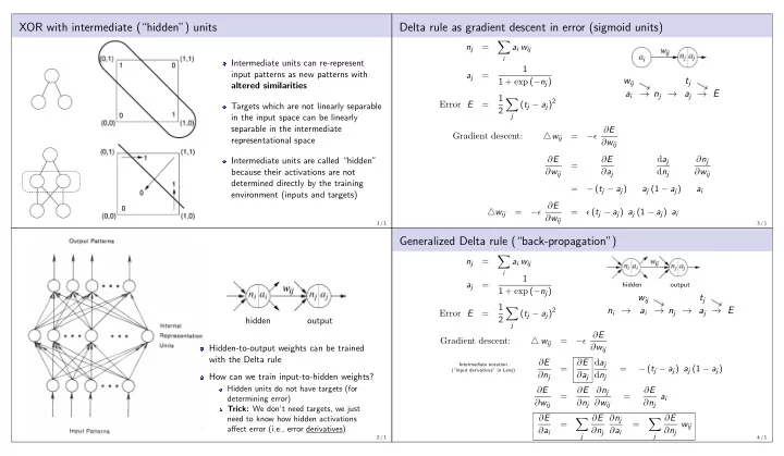
XOR with intermediate (“hidden”) units Delta rule as gradient descent in error (sigmoid units) � n j = a i w ij i Intermediate units can re-represent 1 input patterns as new patterns with a j = w ij t j 1 + exp ( − n j ) altered similarities a i → n j → a j → E 1 ( t j − a j ) 2 � Error E = Targets which are not linearly separable 2 in the input space can be linearly j separable in the intermediate − ǫ ∂ E Gradient descent: △ w ij = representational space ∂ w ij ∂ E ∂ E d a j ∂ n j Intermediate units are called “hidden” = because their activations are not ∂ w ij ∂ a j d n j ∂ w ij determined directly by the training = − ( t j − a j ) a j (1 − a j ) a i environment (inputs and targets) − ǫ ∂ E △ w ij = = ǫ ( t j − a j ) a j (1 − a j ) a i ∂ w ij 1 / 1 3 / 1 Generalized Delta rule (“back-propagation”) � = n j a i w ij i 1 = a j hidden output 1 + exp ( − n j ) w ij t j 1 n i → a i → n j → a j → E � ( t j − a j ) 2 Error E = 2 hidden output j − ǫ ∂ E Gradient descent: △ w ij = Hidden-to-output weights can be trained ∂ w ij with the Delta rule ∂ E ∂ E d a j Intermediate notation = = − ( t j − a j ) a j (1 − a j ) (“input derivatives” in Lens) ∂ n j ∂ a j d n j How can we train input-to-hidden weights? Hidden units do not have targets (for ∂ E ∂ E ∂ n j ∂ E = = a i determining error) ∂ w ij ∂ n j ∂ w ij ∂ n j Trick: We don’t need targets, we just ∂ E ∂ E ∂ n j ∂ E need to know how hidden activations � � = = w ij affect error (i.e., error derivatives) ∂ a i ∂ n j ∂ a i ∂ n j j j 2 / 1 4 / 1

Back-propagation Accelerating learning: Momentum descent Forward pass ( ⇑ ) Backward pass ( ⇓ ) 1 ∂ E a j = = − ( t j − a j ) 1 + exp ( − n j ) ∂ a j � ∂ E ∂ E n j = a i w ij = a j (1 − a j ) ∂ n j ∂ a j i ∂ E ∂ E = a i ∂ w ij ∂ n j 1 ∂ E ∂ E = a i � = w ij 1 + exp ( − n i ) ∂ a i ∂ n j j − ǫ ∂ E � △ w [ t − 1] � △ w ij [ t ] = + α ij ∂ w ij 5 / 1 7 / 1 What do hidden representations learn? “Auto-encoder” network (4–2–4) Plaut and Shallice (1993) Mapped orthography to semantics (unrelated similarities) Compared similarities among hidden representations to those among orthographic and semantic representations Hidden representations “split the (over settling) difference” between input and output similarity 6 / 1 8 / 1

Projections of error surface in weight space Epochs 3-4 Asterisk: error of current set of weights Tick mark: error of next set of weights Solid curve (0): Gradient direction Solid curve (21): Integrated gradient direction (including momentum) This is actual direction of weight step (tick mark is on this curve) Number is angle with gradient direction Dotted curves: Random directions (each labeled by angle with gradient direction) 9 / 1 11 / 1 Epochs 1-2 Epochs 5-6 10 / 1 12 / 1

Epochs 7-8 Epochs 25-50 13 / 1 15 / 1 Epochs 9-10 Epochs 75-end 14 / 1 16 / 1

High momentum (epochs 1-2) High learning rate (epochs 1-2) 17 / 1 19 / 1 High momentum (epochs 3-4) High learning rate (epochs 3-4) 18 / 1 20 / 1