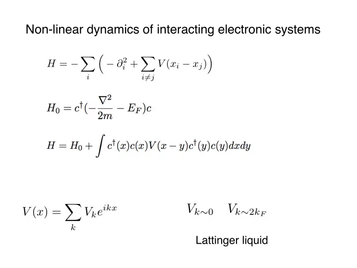
SLIDE 1 Non-linear dynamics of interacting electronic systems
H = − X
i
≥ − ∂2
i +
X
i6=j
V (xi − xj) ¥
Vk∼0 Vk∼2kF
Lattinger liquid
V (x) = X
k
Vkeikx
SLIDE 2
Model Hamiltonian: Elliptic Calogero-Sutherland model
V (x) = ℘(x) → 1 x2 , 1 sinh2 x,
1 sin2 x, ∇δ(x)
Interpolates between Lattinger liquid and Calogero model - quantum wires, edge states of FQHE The last and the major unsolved integrable model
H = X
i
≥ − ∂2
i + λ(λ − 1)
X
j
℘(xi − xj) ¥
SLIDE 3
˙ ϕ + (∂xϕ)2 = 0
Free fermions:
ρ(x) = −∇xϕ = ρ0 + X
k
akeikx [ak, ak0] = kδk+k0, ρk = ρ†
−k
SLIDE 4
˙ ϕ = 1 2(∂xϕ)2 + ∂2
x ˜
ϕ
˜ ϕ = 1 πL Z cot x − x0 L ϕ(x0)dx0
℘(x + iL) = ℘(x)
chiral sector
H = X
i
≥ − ∂2
i + λ(λ − 1)
X
j
℘(xi − xj) ¥
SLIDE 5
Chiral sector - long-time asymptotes of non-linear waves
SLIDE 6
˜ ϕ = 1 πL Z cot x − x0 L ϕ(x0)dx0
L → 0 : ˙ ϕ = 1 2(∂xϕ)2 + ∂3
xϕ
ILW-equation KdV-equation
L → ∞ : ˙ ϕ = 1 2(∂xϕ)2 + ∂2
x
Z ϕ(x0) x − x0 dx0
Benjamin-Ono equation
˙ ϕ = 1 2(∂xϕ)2 + (λ − 1)∂2 ˜ ϕ
SLIDE 7
On the relation between Calogero model and CFT
α0 = √ λ − 1/ √ λ λ(λ − 1) (xi − xj)2 Txy = (∂xϕ)2 + α0∂2
x ˜
ϕ
Flux of energy through the boundary
˙ ϕ = Txy
SLIDE 8
Period of oscillations is
(interaction) × (δρ)−1 >> k−1
F
Quantum Non-linear Equations can be treated semiclassically
SLIDE 9 Trigonometric Calogero-Sutherland model Model for edge states of the FQHE
H = − X
i
∂2
i +
X
j
λ(λ − 1) sin2(xi − xj)
HΨ = EΨ
Ψ(x1, . . . , xN) = Y
i>j
(eixi − eixj)λJY (x1, . . . , xN)
Jack symmetric polynomial
λ = 0 − bosons
λ = 1 − fermions
Ψ(...xi...xj...) = e2πiλΨ(...xj...xi...)
SLIDE 10
H = − X
i
∂2
i +
X
j
λ(λ − 1) sin2(xi − xj)
˙ ϕ = 1 2(∂xϕ)2 + (λ − 1)∂2 ˜ ϕ
ak>0 = X
i
eikxi
[ak, a−k0] = λkδkk0
ϕ(x) = X
k
eikx k ak,
SLIDE 11
Properties: 1) Integrable (despite being non-local); 2) Its solitons carry a quantized fractional charge:
˙ ϕ + (∂xϕ)2 + ν∂2
xϕH = 0
Z ρdx = Z dϕ = integer × ν
3) Solitons have Lorentzian shape:
ρs(x, t) = 1 π vν v2(x − vt)2 + ν2
Properties of Benjamin-Ono Equation
SLIDE 12
Soliton - collective excitation of particles
SLIDE 13
Shock wave:
competition between non-linear term and dispersion term
˙ ϕ + (∂xϕ)2 + ν∂2
xϕH = 0
SLIDE 14
Long time asymptote: Soliton train
SLIDE 15
Soliton Train time
space
SLIDE 16
A single soliton (area is 1/3) 1/4 of quantum (area is 1/12)
SLIDE 17
N=7 N=20
Soliton trains
SLIDE 18
SLIDE 19
Separation between hole (moving right) and particles (moving left)
SLIDE 20
Conclusions:
1) Dynamics of the edge state is essentially non-linear; 2) Solitons of non-linear dynamics carry fractional charge; 3) A propagation of any front evolves to a shock wave and further in a fractionally quantized soliton train. Quantum shocks in BEC
SLIDE 21
SLIDE 22
SLIDE 23
SLIDE 24 Quantum Hydrodynamics of Calogero-Sutherland model
˙ xi = pi
˙ pi = X
j
λ(λ − 1) (xi − xj)3
˙ xi = X
k
λ xi − yk − X
k
λ xi − xk
− ˙ yi = X
k
λ yi − xk − X
k
λ yi − yk
pi = X
k
λ xi − yk − X
k
λ xi − xk
SLIDE 25 ˙ xi = X
k
λ xi − yk − X
k
λ xi − xk − ˙ yi = X
k
λ yi − xk − X
k
λ yi − yk ϕ(z) = λ X
i
log(z − xk) + λ X
i
log(z − yk) ˜ ϕ(z) = λ X
i
log(z − xk) − λ X
i
log(z − yk) ˙ ϕ = 1 2(∂xϕ)2 + (λ − 1)∂2 ˜ ϕ
SLIDE 26
Density and velocity
∂x ≥ ϕ(x + i0) − ϕ(x − i0) ¥ = −2λπρ(x)
∂x ≥ ϕ(x + i0) + ϕ(x − i0) ¥ = v − 2iλ∂x log ρ
˙ ρ + ∂x(ρv) = 0
SLIDE 27 ˙ ρ + ∂x(ρv) = 0
˙ v + ∂x ≥v2 2 + w(ρ) ¥ = 0
w(ρ) = λ2π2 2 ρ2 − λ(λ − 1) 2 1 √ρ∂2
x
√ρ + πλ(λ − 1)∂xρH
ρH(x) = Z coth(x − x0)ρ(x0)dx0
SLIDE 28
v = λ ≥ πρ + ∂x(log √ρ)H¥
ρt + λ∂x ≥ πρ2 + ρ∂x(log √ρ)H¥ = 0
Chiral reduction
two equations become one
Chiral non-linear equation
ρ ≈ ρ0 + u + . . . ˙ u + uux + (λ − 1)˜ uxx = 0
Benjamin-On equation