( x ik x i )( x jk x j ) N Expected value of a vector x is by - PDF document

Up To Higher Dimensions • Our previous Kalman Filter discussion was Lecture 10: of a simple one-dimensional model. Extended Kalman Filters • Now we go up to higher dimensions: n – State vector: x � � CS 344R/393R: Robotics m – Sense vector: z � � Benjamin Kuipers l u � � – Motor vector: • First, a little statistics. Expectations Variance and Covariance • Let x be a random variable. • The variance is E [ ( x - E [ x ]) 2 ] • The expected value E [ x ] is the mean: N 2 ] = 1 2 = E [( x � x � 2 N ) ( x i � x ) � � x = 1 � � N E [ x ] = x p ( x ) dx x i 1 N 1 • Covariance matrix is E [ ( x - E [ x ])( x - E [ x ]) T ] – The probability-weighted mean of all possible N C ij = 1 values. The sample mean approaches it. � ( x ik � x i )( x jk � x j ) N • Expected value of a vector x is by component. k = 1 T E [ x ] = x = [ x 1 , L x n ] – Divide by N − 1 to make the sample variance an unbiased estimator for the population variance. 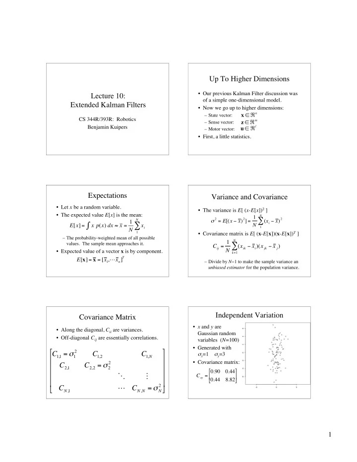Independent Variation Covariance Matrix • x and y are • Along the diagonal, C ii are variances. Gaussian random • Off-diagonal C ij are essentially correlations. variables ( N =100) • Generated with � 2 � C 1,1 = � 1 C 1,2 C 1, N σ x =1 σ y =3 � � • Covariance matrix: 2 C 2,1 C 2,2 = � 2 � � C xy = 0.90 � 0.44 � � � O M � � 0.44 8.82 � � � � 2 L C N ,1 C N , N = � N � � 1

Dependent Variation Discrete Kalman Filter • Estimate the state x ∈ ℜ n of a linear • c and d are random stochastic difference equation variables. x k = Ax k � 1 + Bu k � 1 + w k � 1 • Generated with – process noise w is drawn from N (0, Q ), with c=x+y d=x-y covariance matrix Q . • Covariance matrix: • with a measurement z ∈ ℜ m z k = Hx k + v k C cd = 10.62 � � 7.93 � – measurement noise v is drawn from N (0, R ), with � � � 7.93 8.84 covariance matrix R . � � • A, Q are n × n . B is n × l . R is m × m . H is m × n . Estimates and Errors Time Update (Predictor) n ˆ • is the estimated state at time-step k . x k � � • Update expected value of x � � � n ˆ � = A ˆ x • after prediction, before observation. ˆ x x k � 1 + Bu k � 1 k k � = x k � ˆ • Errors: e k x � • Update error covariance matrix P k � = AP k � 1 A T + Q e k = x k � ˆ x P k k • Error covariance matrices: � T ] � e k � = E [ e k • Previous statements were simplified P k versions of the same idea: T ] P k = E [ e k e k ˆ � ) = ˆ x ( t 3 x ( t 2 ) + u [ t 3 � t 2 ] ˆ • Kalman Filter’s task is to update x P k 2 ( t 3 � ) = � 2 ( t 2 ) + � � 2 [ t 3 � t 2 ] � k Measurement Update (Corrector) The Kalman Gain • Update expected value • The optimal Kalman gain K k is � + K k ( z k � H ˆ � ) ˆ k = ˆ x x x T ( HP k T + R ) k k � H � H � 1 K k = P � z k � H ˆ x k – innovation is k � H T P k • Update error covariance matrix = T + R � � H HP k P k = (I � K k H)P k • Compare with previous form • Compare with previous form � ) + K ( t 3 )( z 3 � ˆ � )) ˆ ( t 3 ) = ˆ x x ( t 3 x ( t 3 � 2 ( t 3 � ) K ( t 3 ) = 2 ( t 3 ) = ( 2 ( t 3 � ) � 1 � K ( t 3 )) � 2 ( t 3 � ) + � 3 2 � 2

The Jacobian Matrix Extended Kalman Filter • For a scalar function y = f ( x ), • Suppose the state-evolution and measurement equations are non-linear: � y = f ( x ) � x � • For a vector function y = f ( x ), x k = f ( x k � 1 , u k � 1 ) + w k � 1 z k = h ( x k ) + v k � � � f 1 � f 1 L ( x ) ( x ) � � � � � � � y 1 � x 1 � x � x n � � – process noise w is drawn from N (0, Q ), with � � � � 1 � � � y = J � x = � M � = M M � � M � covariance matrix Q . � � � � � � � f n � f n – measurement noise v is drawn from N (0, R ), � � � y n � x n � � L � � ( x ) ( x ) with covariance matrix R . � � � x � x n � � 1 Linearize the Non-Linear EKF Update Equations � = f (ˆ x ˆ x k � 1 , u k � 1 ) • Predictor step: • Let A be the Jacobian of f with respect to x . k � = AP k � 1 A T + Q A ij = � f i P k ( x k � 1 , u k � 1 ) � x j T ( HP k T + R ) � H � H � 1 • Kalman gain: K k = P • Let H be the Jacobian of h with respect to x . k H ij = � h i ( x k ) � + K k ( z k � h (ˆ � )) x ˆ k = ˆ x x � x j • Corrector step: k k • Then the Kalman Filter equations are almost � P k = (I � K k H)P k the same as before! Next • Building a map of landmark locations by combining uncertain observations. 3