Chapter 6 Optimal Estimator - Kalman Filter Formulation We want to - PDF document

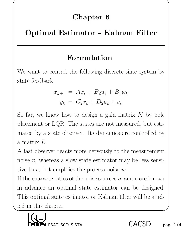
✬ ✩ Chapter 6 Optimal Estimator - Kalman Filter Formulation We want to control the following discrete-time system by state feedback x k +1 = Ax k + B 2 u k + B 1 w k y k = C 2 x k + D 2 u k + v k So far, we know how to design a gain matrix K by pole placement or LQR. The states are not measured, but esti- mated by a state observer. Its dynamics are controlled by a matrix L . A fast observer reacts more nervously to the measurement noise v , whereas a slow state estimator may be less sensi- tive to v , but amplifies the process noise w . If the characteristics of the noise sources w and v are known in advance an optimal state estimator can be designed. This optimal state estimator or Kalman filter will be stud- ied in this chapter. ✫ ✪ CACSD pag. 174 ESAT–SCD–SISTA

✬ ✩ Discrete-time Kalman filtering Least squares formulation Consider a discrete-time system x k +1 = Ax k + B 2 u k + B 1 w k y k = C 2 x k + D 2 u k + v k . At a certain time k , the state space equations can be as- sembled in a large over-determined set of linear equations, with a vector of unknowns θ containing all previous state vectors, up to x k +1 :       − B 2 u 0 A − I B 1 w 0   x 0       y 0 − D 2 u 0 C 2 0 v 0             x 1           − B 2 u 1 − I A B 1 w 1           x 2         = + y 1 − D 2 u 1 0 C 2 v 1       .   .       .   . . ...  .     .  . .           x k         − B 2 u k A − I B 1 w k             x k +1 y k − D 2 u k 0 C 2 v k � �� � θ � �� � � �� � � �� � e A b ✫ ✪ CACSD pag. 175 ESAT–SCD–SISTA

✬ ✩ We have to find an optimal state vector estimate ˆ θ that is the ’best’ solution for the set of equations b = A θ + e . Vector e contains stacked and weighted noise samples w k and v k . We assume that the characteristics of w and v are known and are such that E ( e ) = 0 : zero-mean E ( ee T ) = W W is the so-called noise covariance matrix, which in this case gives some information about the amplitude of the noise components, their mutual correlation and spectral shaping (correlation in time domain). If the components of both w and v are stationary, mutually uncorrelated and white, having the same variance σ 2 w and σ 2 v respectively,   σ 2 w B 1 B T 0 0 0 . . . 1   σ 2 0 0 0 v I . . .     σ 2 w B 1 B T W = 0 0 0 1 . . .     . . ... ... ... . .   . .   . . . σ 2 0 0 0 v I ✫ ✪ CACSD pag. 176 ESAT–SCD–SISTA

✬ ✩ The optimal estimate for θ can be found as ˆ θ = ( A T W − 1 A ) − 1 A T W − 1 b ˆ θ is the least squares solution to θ { ( b − A θ ) T W − 1 ( b − A θ ) } min based on input-output data up to time k . Disadvantage: k → ∞ ⇒ dimension of A → ∞ . ✫ ✪ CACSD pag. 177 ESAT–SCD–SISTA

✬ ✩ Recursive least squares problem Finite horizon case : How can we find an optimal estimate ˆ x k +1 | k , in the least squares sense, for the state x k +1 , by making use of observa- tions of inputs u and outputs y up to time k , given ˆ x k | k − 1 , the estimate for x k at time k − 1 ? Consider the following state observer x k +1 | k = A ˆ ˆ x k | k − 1 + B 2 u k + L k ( y k − C 2 ˆ x k | k − 1 − D 2 u k ) . Combining it with the system equations leads to the esti- mator error equation x k +1 | k = x k +1 − ˆ ˜ x k +1 | k = ( A − L k C 2 )˜ x k | k − 1 + B 1 w k − L k v k We will assume that w k and v k have zero-mean white noise characteristics with covariance E ( w j w T k ) = Qδ jk , E ( v j v T k ) = Rδ jk , E ( v j w T k ) = 0 and Q and R nonnegative definite weighting matrices. ✫ ✪ CACSD pag. 178 ESAT–SCD–SISTA

✬ ✩ Our aim now is to find an optimal estimator gain L k that minimizes α T P k +1 α = α T E ((˜ x k +1 )) T ) α. x k +1 − E (˜ x k +1 ))(˜ x k +1 − E (˜ α is an arbitrary column vector. P k is called the estimation error covariance matrix. From the estimator error equation and taking in account the properties of the noise : E (˜ x k +1 ) = ( A − L k C 2 ) E (˜ x k ) . Now if we take E (˜ x 0 ) = 0, the mean value of the estimation error is zero for all k . Then, x k +1 ) T ) P k +1 = E ((˜ x k +1 )(˜ = ( A − L k C 2 ) P k ( A − L k C 2 ) T + B 1 QB T 1 + L k RL T k So, if P 0 is properly set, P k will be symmetric positive semidefinite for all k . ✫ ✪ CACSD pag. 179 ESAT–SCD–SISTA

✬ ✩ The optimal L k or Kalman filter gain can be obtained by minimizing α T P k +1 α. L k = argmin L k Setting the derivative with respect to L k equal to zero, α T ( − 2 AP k C T 2 + 2 L k ( R + C 2 P k C T 2 )) α = 0 . The equality has to be fulfilled for all vectors α , so L k = AP k C T 2 ( R + C 2 P k C T 2 ) − 1 . and the error covariance update equation becomes P k +1 = AP k A T + B 1 QB T 1 − AP k C T 2 ( R + C 2 P k C T 2 ) − 1 C 2 P k A T which is a Riccati difference equation. ✫ ✪ CACSD pag. 180 ESAT–SCD–SISTA

✬ ✩ Infinite horizon case : It can be shown that if the system is controllable and ob- servable and k → ∞ , matrix P k converges to a steady-state positive semidefinite matrix P and L k approaches a con- stant matrix L with 2 ) − 1 . L = APC T 2 ( R + C 2 PC T P satisfies the Discrete Algebraic Riccati Equation : 1 + APA T − APC T 2 ) − 1 C 2 PA T P = B 1 QB T 2 ( R + C 2 PC T Both for the finite horizon and the infinite horizon case, the Kalman filter equations are similar to the equations we obtained for LQR design. ✫ ✪ CACSD pag. 181 ESAT–SCD–SISTA

✬ ✩ Verify the duality relation between Kalman filter design and LQR by using the following conversion table and plugging in the correct matrices in the LQR equations. Conversion table LQR ↔ Kalman filter design LQR Kalman filter A T A C T B 2 B 1 QB T Q 1 L T K Kalman filters may be designed based on LQR formulas using this table, as is done in Matlab for instance. The Kalman filter is sometimes referred to as LQE, i.e. a Linear Quadratic Estimator. ✫ ✪ CACSD pag. 182 ESAT–SCD–SISTA

✬ ✩ Continuous-time Kalman filtering Consider a system: x = Ax + B 2 u + B 1 w, ˙ y = C 2 x + D 2 u + v and the estimator: ˙ x = A ˆ ˆ x + L ( y − C 2 ˆ x − D 2 u ) + B 2 u where the input disturbance noise w and the sensor noise v are zero mean white noise with covariance Q and R re- spectively. Find an optimal L such that the following stochastic cost function � 1 � T �� � x ) T ( x − ˆ E ( x − ˆ x ) dt T 0 is minimized. ✫ ✪ CACSD pag. 183 ESAT–SCD–SISTA

✬ ✩ Finite-horizon case : This leads to the Riccati differential equation : P = PA T + AP − PC T − ˙ 2 R − 1 C 2 P + B 1 QB T P (0) = 0 . 1 , The optimal estimator or Kalman gain : 2 R − 1 L = P ( t ) C T Infinite-horizon case : This leads to the continuous Algebraic Riccati equation : PA T + AP − PC T 2 R − 1 C 2 P + B 1 QB T 1 = 0 and the corresponding Kalman gain : L = PC T 2 R − 1 Duality with LQR design : Also for the continuous time case the conversion rules on page 182 hold. ✫ ✪ CACSD pag. 184 ESAT–SCD–SISTA

✬ ✩ Examples of Kalman Filter Design Example Boeing 747 aircraft control - Kalman Filter Suppose the plant noise w enters the system in the same way as the control input and suppose the measurement noise is v . Then x = Ax + Bu + B 1 w, ˙ y = Cx + Du + v. where ( A, B, C, D ) is the nominal aircraft model given in � � T the previous examples. B 1 = B = . Sup- 1 0 0 0 0 0 pose further that w and v are white noises with the covari- ance of w , R w = 0 . 7 and the covariance of v R v = 1. The Riccati equation QA T + AQ − QC T R − 1 v CQ + B 1 R w B T 1 = 0 ✫ ✪ CACSD pag. 185 ESAT–SCD–SISTA

✬ ✩ has a solution:   3 . 50 e − 2 1 . 94 e − 3 − 1 . 60 e − 2 2 . 88 e − 3 − 3 . 08 e − 4 − 1 . 55 e − 3   1 . 94 e − 3 5 . 20 e − 1 3 . 68 e − 2 − 9 . 45 e − 1 3 . 43 e + 0 − 3 . 88 e − 2      − 1 . 60 e − 2 3 . 68 e − 2 8 . 18 e − 1 − 6 . 79 e − 1  1 . 34 e + 1 1 . 78 e + 0   Q =   2 . 88 e − 3 − 9 . 45 e − 1 − 6 . 79 e − 1 5 . 06 e + 0 − 1 . 03 e + 0 1 . 59 e − 1      − 3 . 08 e − 4 1 . 34 e + 1 − 1 . 03 e + 0  3 . 43 e + 0 3 . 51 e + 2 4 . 12 e + 1   − 1 . 55 e − 3 − 3 . 88 e − 2 1 . 78 e + 0 1 . 59 e − 1 4 . 12 e + 1 5 . 33 e + 0 and the Kalman filter gain is   − 1 . 5465 e − 02   4 . 9686 e − 02       2 . 2539 e − 01 L = QC T R − T   = .   v − 7 . 3199 e − 01     − 3 . 0200 e − 01     − 8 . 2157 e − 15 Now we can compare this result with the result from pole placement discussed in the previous chapter. The Kalman Filter has poles at − 9 . 992 , − 0 . 1348 ± 0 . 9207 i, − 0 . 5738 , − 0 . 0070 , − 0 . 352 They are slower than those from pole placement, but the Kalman filter is less (actually least) sensitive to the noises. ✫ ✪ CACSD pag. 186 ESAT–SCD–SISTA