Page 1
EKF, UKF
Pieter Abbeel UC Berkeley EECS
Many slides adapted from Thrun, Burgard and Fox, Probabilistic Robotics
n
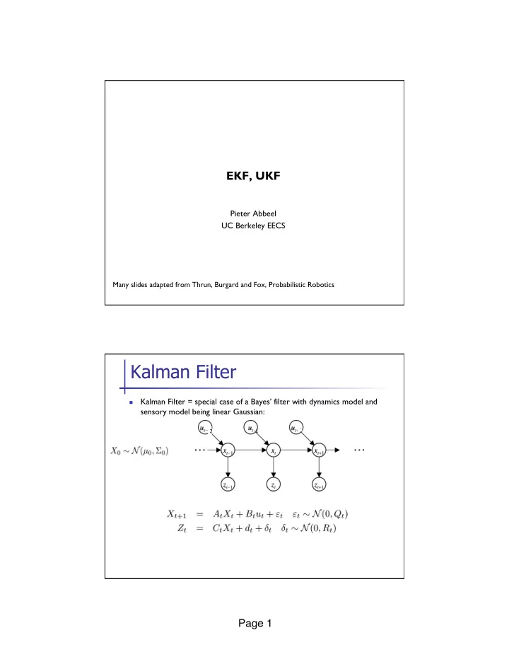
Kalman Filter = special case of a Bayes’ filter with dynamics model and sensory model being linear Gaussian:
Kalman Filter
2
- 1

Kalman Filter Kalman Filter = special case of a Bayes filter with - - PDF document
EKF, UKF Pieter Abbeel UC Berkeley EECS Many slides adapted from Thrun, Burgard and Fox, Probabilistic Robotics Kalman Filter Kalman Filter = special case of a Bayes filter with dynamics model and n sensory model being linear Gaussian: 2
Pieter Abbeel UC Berkeley EECS
Many slides adapted from Thrun, Burgard and Fox, Probabilistic Robotics
n
Kalman Filter = special case of a Bayes’ filter with dynamics model and sensory model being linear Gaussian:
2
n At time 0: n For t = 1, 2, …
n Dynamics update: n Measurement update:
4
n Most realistic robotic problems involve nonlinear functions:
n Versus linear setting:
5
6
“Gaussian of p(y)” has mean and variance of y under p(y)
7
8
p(x) has high variance relative to region in which linearization is accurate.
9
p(x) has small variance relative to region in which linearization is accurate.
10 n Dynamics model: for xt “close to” µt we have: n Measurement model: for xt “close to” µt we have:
n Numerically compute Ft column by column:
n Here ei is the basis vector with all entries equal to zero,
n If wanting to approximate Ft as closely as possible then ²
n Given: samples {(x(1), y(1)), (x(2), y(2)), …, (x(m), y(m))} n Problem: find function of the form f(x) = a0 + a1 x that fits
n Recall our objective: n Let’s write this in vector notation:
n
n Set gradient equal to zero to find extremum:
(See the Matrix Cookbook for matrix identities, including derivatives.)
n For our example problem we obtain a = [4.75; 2.00]
n More generally: n In vector notation:
n
n Set gradient equal to zero to find extremum (exact same
0 10 20 30 40 10 20 30 20 22 24 26
n So far have considered approximating a scalar valued function from
n A vector valued function is just many scalar valued functions and
n In our vector notation: n This can be solved by solving a separate ordinary least squares
n Solving the OLS problem for each row gives us: n Each OLS problem has the same structure. We have
n Approximate xt+1 = ft(xt, ut)
{( xt(1), y(1)=ft(xt(1),ut), ( xt(2), y(2)=ft(xt(2),ut), …, ( xt(m), y(m)=ft(xt(m),ut)}
n Similarly for zt+1 = ht(xt)
n OLS vs. traditional (tangent) linearization:
n Perhaps most natural choice:
n n reasonable way of trying to cover the region with
n Numerical (based on least squares or finite differences) could
n Computational efficiency:
n Analytical derivatives can be cheaper or more expensive
n Development hint:
n Numerical derivatives tend to be easier to implement n If deciding to use analytical derivatives, implementing finite
n At time 0: n For t = 1, 2, …
n Dynamics update: n Measurement update:
34
n Highly efficient: Polynomial in measurement dimensionality k
n Not optimal! n Can diverge if nonlinearities are large! n Works surprisingly well even when all assumptions are
35
36
37
n
Assume we know the distribution over X and it has a mean \bar{x}
n
Y = f(X)
n
EKF approximates f by first order and ignores higher-order terms
n
UKF uses f exactly, but approximates p(x).
[Julier and Uhlmann, 1997]
n When would the UKF significantly outperform the EKF?
n Analytical derivatives, finite-difference derivatives, and least squares
will all end up with a horizontal linearization à they’d predict zero variance in Y = f(X)
Beyond scope of course, just including for completeness.
A crude preliminary investigation of whether we can get EKF to match UKF by particular choice of points used in the least squares fitting
n
Picks a minimal set of sample points that match 1st, 2nd and 3rd moments
n
\bar{x} = mean, Pxx = covariance, i à i’th column, x 2 <n
n
· : extra degree of freedom to fine-tune the higher order moments of the approximation; when x is Gaussian, n+· = 3 is a suggested heuristic
n
L = \sqrt{P_{xx}} can be chosen to be any matrix satisfying:
n L LT = Pxx
[Julier and Uhlmann, 1997]
n Dynamics update:
n Can simply use unscented transform and estimate the
n Observation update:
n Use sigma-points from unscented transform to compute
[Table 3.4 in Probabilistic Robotics]
n Highly efficient: Same complexity as EKF, with a constant factor
n Better linearization than EKF: Accurate in first two terms of
n Derivative-free: No Jacobians needed n Still not optimal!