Workshop exercise Data integration and analysis In this exercise, - PDF document

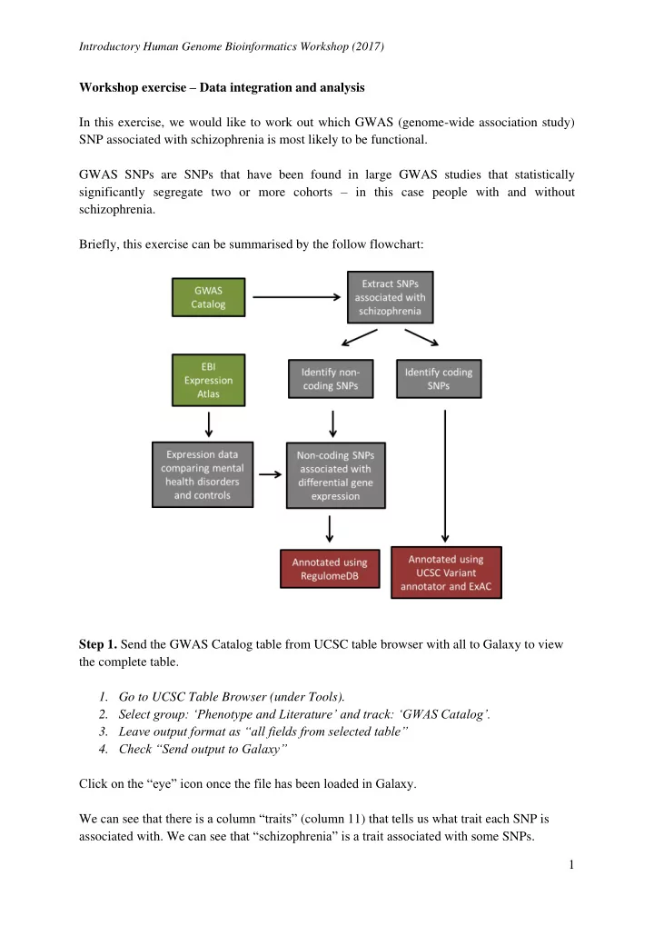
Introductory Human Genome Bioinformatics Workshop (2017) Workshop exercise – Data integration and analysis In this exercise, we would like to work out which GWAS (genome-wide association study) SNP associated with schizophrenia is most likely to be functional. GWAS SNPs are SNPs that have been found in large GWAS studies that statistically significantly segregate two or more cohorts – in this case people with and without schizophrenia. Briefly, this exercise can be summarised by the follow flowchart: Step 1. Send the GWAS Catalog table from UCSC table browser with all to Galaxy to view the complete table. 1. Go to UCSC Table Browser (under Tools). 2. Select group: ‘Phenotype and Literature’ and track: ‘GWAS Catalog’. 3. Leave output format as “all fields from selected table” 4. Check “Send output to Galaxy” Click on the “eye” icon once the file has been loaded in Galaxy. We can see that there is a column “traits” (column 11) that tells us what trait each SNP is associated with. We can see that “ s chizophrenia” is a trait associated with som e SNPs. 1

Introductory Human Genome Bioinformatics Workshop (2017) Step 2. Go to Galaxy and import GWAS Catalog SNPs associated with Schizophrenia traits. To keep this simple, we will just select traits that start with the word “ Schizophrenia ”. 1. Go to ‘Get Data’ and ‘UCSC Main table browser’ 2. Select ‘GWAS Catalog’ track as above. 3. To get only SNPs associated with ‘ Schizophrenia ’, click on the ‘create’ button next to ‘filter’ and type “ Schizophrenia ” in the trait text box. This will retrieve any SNP that begins with the word “ Schizophrenia ” in the trait column. 4. Make sure ‘output format’ is ‘BED’ then send query to Galaxy The dataset should have 999 SNPs. Step 3. Now to identify gene exons associated with the SNPs, we need to obtain the exonic regions of the human genome. To do this, import genic regions from the UCSC genome browser. 1. Go to ‘Get Data’ and ‘UCSC Main table browser’ 2. Select group: ‘Genes and Gene Predictions’ and track: ‘RefSeq Genes’. 3. Select table: ‘refFlat’ 4. Make sure ‘output format’ is ‘BED’ then click get output 5. Select ‘Coding Exons’ and click Send query to Galaxy refFlat is a handy table because it uses official gene symbols rather than accession numbers as the gene ID. Step 4. Identify schizophrenia SNPs that are within coding exons 1. Use ’ Join ’ under ‘Operate on Genomic Intervals’ 2. We are interested in the genes, so put the refFlat genes as dataset 1 and the SNPs as dataset2 There should be 33 exons overlapping SNPs. Notice that some SNPs are listed multiple times. This is because refFlat contains multiple transcript, so some SNPs overlap multiple exons of transcripts. We will deal with the duplicates later. Step 5. The rest of the SNPs fall in non-coding regions. These SNPs may affect gene regulation, therefore we are interested to find out which genes may be affected. Working out which gene may be regulated is rudimentarily done by proximity to the SNP. To do this we first identify SNPs that fall within non-coding regions. To get the non-coding regions: 1. Use ’Complement’ under ‘Operate on Genomic Intervals’ 2

Introductory Human Genome Bioinformatics Workshop (2017) 2. Select the refFlat dataset to complement. 3. Select Yes to ‘Genome - wide complement’. To identify non-coding SNPs: 1. Use ’Intersect’ under ‘Operate on Genomic Intervals’ 2. This time we are interested in the SNPs (in order to work out what gene is close to the SNPs), so put the SNPs as dataset 1 and the complement (non-coding) regions in dataset 2. There should be 978 non-coding SNPs. To identify genes closest to(and therefore potentially regulated by) the SNPs: 1. Use ’ Fetch closest non-overlapping feature ’ under ‘Operate on Genomic Intervals’ 2. Select the intergenic SNPs as the first dataset and the refFlat genes as the second dataset. 3. Keep ‘Located’ as ‘Either Upstream and Downstream’ as we just want the closest exon (which contains the gene name). 4. As the gene name is embedded with the exon information in column 8, to make the gene name into a column for easier downstream processing use “Convert” from “Text Manipulation”. Select Convert all “Underscores” to the non -coding SNP file. There should still be 978 entries but now the closest gene name is shown in column 8 Step 6. We now want to see whether any of our schizophrenia non-coding SNPs are also differentially expressed genes. To do this we first need to find a dataset that has compared the gene expression profiles of people with schizophrenia and control. There may be many such datasets, but today we will use the EBI Expression Atlas to retrieve the data. The EBI Expression Atlas contains processed datasets that have gone through a curated process and therefore in theory should be more reliable. 1. Browse to https://www.ebi.ac.uk/gxa/home 2. Select ‘Homo sapiens’ and type ‘ mental or behavioural disorder ’ (schizophrenia also works, but for the purpose of this tutorial it is too restrictive) in the ‘Sample properties’ text box and hit search. 3. Expression Atlas shows a list of differentially expressed genes identified from all curated studies relating to comparing different forms of mental health disorder (mostly bipolar) to ‘normal’ samples. 3

Introductory Human Genome Bioinformatics Workshop (2017) 4. Download these differentially expressed genes and save to computer (i.e. Desktop) Click here to download 5. Upload the downloaded file to Galaxy. Select ‘tabular’ for the format of the file. Step 7. We can now use Galaxy to find out the overlap between the schizophrenia associated SNPs and the differentially expressed genes. But unfortunately, as is often the case when doing bioinformatics, the gene names from EBI Expression Atlas are Ensembl GeneIDs where as our gene names are HUGO gene names. So we have to first map the Ensembl IDs to gene names. 1. To download HUGO gene name to Ensembl GeneID map from UCSC, first go to UCSC Table browser via Galaxy Get Data. 2. Select Ensembl Genes track from “Gene and Gen Predictions” and select the “ensemblToGeneName” table. 3. For “output format” select “selected fields from primary and related tables” and hit get output. 4. Check ‘ensGtp’ in the Linked Tables and click “allow selection from checked tables. 5. Check “alternate gene name” from the hg19.ensemblToGeneName table at the top and then “ gene ” (Ensembl gene ID) from the hg19.ensGtp table. Click “done with selections” and send to Galaxy. 6. There are many duplicate entries in the ensemble to HUGO gene name map file, so use “ Unique ” (NOT Unique lines) under “ Text Manipulation ” to remove duplicates first. 4

Introductory Human Genome Bioinformatics Workshop (2017) 5

Introductory Human Genome Bioinformatics Workshop (2017) 7. Use “Join two Datasets” from ‘Join, Subtract and Group’ to join differential gene expression file with HUGO gene names. Select differential gene expression file as the first file (using column 1) and the ensemble gene name map table as the second file (using column 2). 8. Finally u se ‘Join two Datasets’ from ‘Join, Subtract and Group’ to join the schizophrenia non-coding SNP and the differentially expressed genes now with gene names in column 8. Make sure to select column 8 for both datasets as that is where the gene name is There should be 2 genes. PDE4B and PTGS2 are both up-regulated log 2.6 fold in bipolar disorder and the associated SNPs are rs12129719 and rs10911092, respectively. Step 8. We can now look at these two SNPs using regulomeDB to see if they really have much potential of altering the expression of PDE4B and PTGS2 1. Go to regulomeDB (http://regulomedb.org/) 2. Paste in rs12129719 and rs10911092 and submit. Unfortunately, neither look like very promising candidates as they both have a regulomeDB score of 6 which is the lowest priority. Step 9. In this final step, we use the UCSC Variant Annotation Integrator to annotate the coding SNPs. 1. Get a list of unique coding SNPs using “Group” from “Join, Subtract and Group” selecting column 10 from the coding SNP dataset (should be dataset 4 in Galaxy in this exercise if you started with a blank session). 2. Go to the UCSC genome browser and bring up the ‘Variant Anntation Integrator’ tool (http://genome.ucsc.edu/cgi-bin/hgVai) for the coding SNPs. 3. Under s elect variants, change ‘Artificial Example Variants’ to ‘Variant identifiers’. Type or paste in the list of 8 SNPs. 4. There are many options for annotating the SNPs, we will just go with the default setting which includes SIFT and PolyPhen-2 as the most commonly used scoring algorithms for SNPs. 5. Change the output format to ‘Variant Effect Predictor (HTML)’ There are a number of missense SNPs, but rs16897515 is predicted to be damaging by all both SIFT and the two PolyPhen methods. We can also look at this SNP is ExAC, which shows that it has a relatively high allele frequency (>15%) in the population. 6