Why? performance wise not!! 3 4 The inner loop of matrix Matrix - - PDF document

1

Lecture 9: Numerical Algorithms and Pipelining

2

Numerical Algorithms

• Solve big linear equation systems

– Dense – Sparse

• Optimization
• Iterative methods
• FFT

etc.

3

BLAS Level 1, 2, and 3

• BLAS 1

– operates on vectors (1D), saxpy, scaling, rotations,...

• BLAS 2

– operates on matrix (2D), matrix vector

• BLAS 3

– operates on pairs or triplets of matrices, matrix-matrix

• Mathematically are many of these equivalent,

performance wise not!!

Why?

4

Because!

Routine #Flops #mem. refs

daxpy 2n 2n dgemv 2n2 n2 dgemm 2n3 3n2

5

Matrix multiplication: IJK

for i = 1, n for j = 1, n for k = 1, n C(i,j) = C(i,j) + A(i,k) * B(k,j) end end end

C A B k k The inner loop computes c(i, j) = dotproduct(A(i,.:), B(:, j))

6

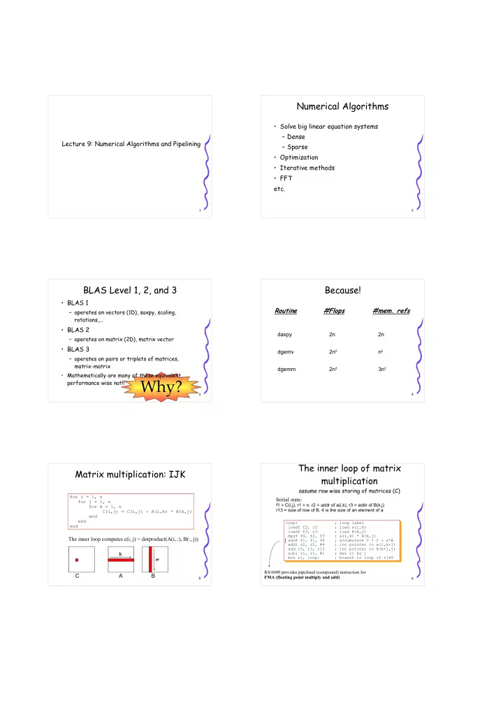
The inner loop of matrix multiplication

assume row wise storing of matrices (C)

loop: ; loop label loadf f2, r2 ; load a(i,k) loadf f3, r3 ; load B(k,j) mpyf f4, f2, f3 ; a(i,k) * B(k,j) addf f1, f1, f4 ; accumulate C = C + a*B addi r2, r2, #4 ; inc pointer to a(i,k+1) add r3, r3, r13 ; inc pointer to B(k+1,j) subi r1, r1, #1 ; dec r1 by 1 bnz r1, loop: ; branch to loop if r1≠0

Initial state:

f1 = C(i,j), r1 = n, r2 = addr of a(i,k), r3 = addr of B(k,j) r13 = size of row of B, 4 is the size of an element of a RS/6000 provides pipelined (compound) instruction for FMA (floating point multiply and add)

{

7

Cache Properties

• Assume row wise storing of matrices (C)
• The inner loop fetches a whole row of A, a

whole column of B

• One row may be larger than the cache

– 128KB cache = 32KWords = 16K double

• One column of B occupies s*n words

– s is the size of the cache line – The inner loop use 1 word from each fetched cache line – Fills the cache with lots of data not used

8

Matrix Multiplication: IKJ-optimization

gives a better spatial locality

for i = 1, n for k = 1, n for j = 1, n C(i,j) = C(i,j) + A(i,k) * B(k,j) end end end

C A B All references in the inner loop are Stride 1; (refer to consecutive memory addresses) Stride 1 j j

9

Matrix Multiplication:

Column Blocked

C A B do jb = 1, n, bs do i = 1, n do j = jb, jb+bs-1 do k = 1, n c(i,j) = c(i,j) + a(i,k)*b(k,j) end Assume the cache can hold one column block of C and B and

• ne row from A

10

Improve Temporal Locality

block for better cache usage

• Transform one multiplication to

multiplications of submatrices

• The sizes of the submatrices is chosen such that

they fit in the cache

–m x m submatrices –2m3 flops for 3m2 data in cache

• Each word fetched to the cache is used m times

C11 C12 C13 C21 C22 C23 C31 C32 C33 A11 A12 A13 A21 A22 A23 A31 A32 A33 B11 B12 B13 B21 B22 B23 B31 B32 B33 = *

C11 = A11*B11 + A12*B21 + A13*B31

11

do ib = 1, n, bs do jb = 1, n, bs do kb = 1, n , bs do i = ib, min(ib+bs, n) do k = kb, min(kb+bs, n) do j = jb, min(jb+bs, n) C(i,j) = C(i,j) + A(i,k) * B(k,j) end end end end end end

Matrix Multiplication: blocked

C A B ib jb ib kb kb jb bs Want C to be in the cache as long as possible

12

Blocked Matrix Multiplication

• The ib, jb, kb loops steps between submatrices
• The i, j, k loops performs a matrix multiplication
• n submatrices
• bs is the block size
• The i, j, k loops are optimized for fast execution
• The ib, jb, kb loops are optimized for cache reuse

– the kb loop reuses one C block – new A and B blocks are fetched to the cache

• For example on performance, see the Master's

Thesis cacheprobe

13

Parallel Matrix Multiplication for

Distributed Memory Message Passing Machine

• Static, but optimal load balancing

– Each processor computes the same number of elements of C

• Coordination/synchronizing
• Initial data distribution

– 1D (the nodes are organized in 1D, (0:p-1))

• Each node stores A and one block column of B and C
• Each node stores one block row of A, B, C
• Each node stores one block row of A and C and one block

column of B

– 2D (the nodes are organized in 2D, (i,j) i = 1:√P, j = 1:√P)

• Each node stores n/√P blocks of A, B, and C

14

Parallel Matrix Multiplication

Several copies of A, block column of B and C Let p = 4 Original data distribution B,C A p1 p2 p3 p4 All

Extra space required to store a copy of A

C = A * B Local computation

15

Parallel Matrix Multiplication

Each node stores one block row of A and C and one block column of B Overlap communication/computation? Next = mod(me+1,p) Prev = mod(p+me-1,p) for i = 1:p C = C + A*B send(B, Next) receive(B, Prev) end

Local computation “No extra space needed”

However there is need for buffer space (user or system)

Communication

B: p send & receive of nx (n/p) elements

A, C B Assume 4 processors in a ring Original data distribution

17

Idea Shift blocks of A along rows Shift blocks of B along columns

Parallel Matrix Multiplication

2D-blocking (Cannon’s algorithm)

Let p = 16 Original data distribution Processor (i,j) stores Aij, Bij, Cij

A00 B00 A01 B01 A02 B02 A03 B03 A10 B10 A11 B11 A12 B12 A13 B13 A20 B20 A21 B21 A22 B22 A23 B23 A30 B30 A31 B31 A32 B32 A33 B33

18

Parallel Matrix Multiplication

2D-blocking (Cannon’s algorithm)

A00 B00 A01 B01 A02 B02 A03 B03 A10 B10 A11 B11 A12 B12 A13 B13 A20 B20 A21 B21 A22 B22 A23 B23 A30 B30 A31 B31 A32 B32 A33 B33 A00 B00 A01 B11 A02 B22 A03 B33 A11 B10 A12 B21 A13 B32 A10 B03 A22 B20 A23 B31 A20 B02 A21 B13 A33 B30 A30 B01 A31 B12 A32 B23

1

A01 B10 A02 B21 A03 B32 A00 B03 A12 B20 A13 B31 A10 B02 A11 B13 A23 B30 A20 B01 A21 B12 A22 B23 A30 B00 A31 B11 A32 B22 A33 B33

2

A02 B20 A03 B31 A00 B02 A01 B13 A13 B30 A10 B01 A11 B12 A12 B23 A20 B00 A21 B11 A22 B22 A23 B33 A31 B10 A32 B21 A33 B32 A30 B03

3

A03 B30 A00 B01 A01 B12 A02 B23 A10 B00 A11 B11 A12 B22 A13 B33 A21 B10 A22 B21 A23 B32 A20 B03 A32 B20 A33 B31 A30 B02 A31 B13

4

19

Parallel Matrix Multiplication

2D-blocking (Cannon’s algorithm)

shift(B, MY_COL) shift(A, MY_ROW) for i = 1:Q C = C + A*B shift(A, MY_ROW) shift(B, MY_COL) end

• “No extra space needed”

– However, there is a need for buffer space (user or system)

• Initial communication

– shift A, B: (n/√p)x(n/√p) elements

• Additional Communication

– shift A, B: (n/√p)x(n/√p) elements

20

More about uniprocessors

for i = 1, n for j = 1, n for k = 1, n C(i,j) = C(i,j) + A(i,k) * B(k,j) end end end How do you do this on a super scalar processor?? I.e., when we want to do more than one (2-4) operations per cycle?

21

Kernel

for i = 1, n for j = 1, n T = C(i,j) for k = 1, n T += A(i,k) * B(k,j) end C(i,j) = T end end How well is this going on a super scalar processor with a ”long pipe”?? I.e., when we want to fill the pipeline as much as possible?

22

Solution: Outer loop unroll

for i = 1, n, 2 for j = 1, n, 2 T11..T22 = C(i,j)..C(i+1,j+1) for k = 1, n T11 += A(i ,k) * B(k,j ) T12 += A(i ,k) * B(k,j+1) T21 += A(i+1,k) * B(k,j ) T22 += A(i+1,k) * B(k,j+1) end C(i,j)..C(i+1,j+1) = T11..T22 end end

23

Preloading

for i = 1, n for j = 1, n T11..T22 = C(i,j)..C(i+1,j+1) for k = 1, n load A(i,k+1), B(k+1,j)... T11 += A(i ,k) * B(k,j ) T12 += A(i+1,k) * B(k,j+1) T21 += A(i ,k) * B(k,j ) T22 += A(i+1,k) * B(k,j+1) end C(i,j)..C(i+1,j+1) = T11..T22 end end

24

Prefetching

• Also called ”algorithmic preloading”
• Load the next set of blocks that are going to

be multiplied – can be made into temporary variables by the programmer, or in the

• bject code by the compiler
• O(n2) data accesses / O(n3) compute steps

25

Recursion

• The research group from Umeå are pioneers
• Recursive data format
• Recursive algorithms

– SMP parallelism appears by it self

26

Gaussian elimination

• Pipelining
• Broadcast
• Cycling

striping

27

Iterative Methods

• Used to solve sparse equation systems
• Utilizes numerical principles
• Example: heat distribution (Laplace's Equation)

28

Laplace’s Equation

• Wants to find a solution to a partial

differential equation

• Finite difference method
• Computation molecule

29

Laplace’s Equation

• After approx. and rewrites (see the book)
• Iteratively:

30

Natural ordering

• Put the

points as you allocate elements in a matrix

31

Relation to linear equation systems

32

Gauss-Seidel Relaxation

33

Red-Black Ordering

34

Multigrid

Next step: finite- element-methods

35

Pipelining

• Divide a problem into a series of tasks
• Each task can be solved by one processor
• The base for all sequential programs
• Pipeline
• Hide latency/communication

36

Pipelining – example

for (i = 0; i < n; i++) sum = sum + a[i] * b[i]; sum = sum + a[0] * b[0]; sum = sum + a[1] * b[1]; sum = sum + a[2] * b[2]; sum = sum + a[3] * b[3]; sum = sum + a[4] * b[4];

37

Pipelining

Three cases when pipelining should be considered: 1) More than one instance of the complete problem is to be executed 2) A series of data items must be processed, each requiring multiple operations 3) Information to start the next process can be passed forward before the process has completed all its internal operations

38

Type 1

An example is vector operations on processors with more than one functional unit

39

Type 2

Sorting

40

Type 2

41

Type 3

Solving a linear equation system

42

Type 3

43

Övningsuppgifter

• Vad är ”the minimal set of MPI routines”?
• När bör man överväga pipelining?
• Härled ett uttryck för den parallella

exekveringstiden och speedup för Cannons algoritm för matrismultiplikation. Antag cut-through routing! Är algoritmen kostnadsoptimal?