[PPT] - What is SQL? Declarative Say what to do rather than how to do it PowerPoint Presentation

SLIDE 1

1

Introduction to SQL

Introduction to databases CSCC43 Winter 2011 Ryan Johnson

Thanks to Arnold Rosenbloom and Renee Miller for material in these slides

2

What is SQL?

Declarative

– Say “what to do” rather than “how to do it”

Avoid data‐manipulation details needed by procedural languages

– Database engine figures out “best” way to execute query

Called “query optimization”
Crucial for performance: “best” can be a million times faster than “worst”
Data independent

– Decoupled from underlying data organization

Views (= precomputed queries) increase decoupling even further
Correctness always assured… performance not so much

– SQL is standard and (nearly) identical among vendors

Differences often shallow, syntactical

Fairly thin wrapper around relational algebra

3

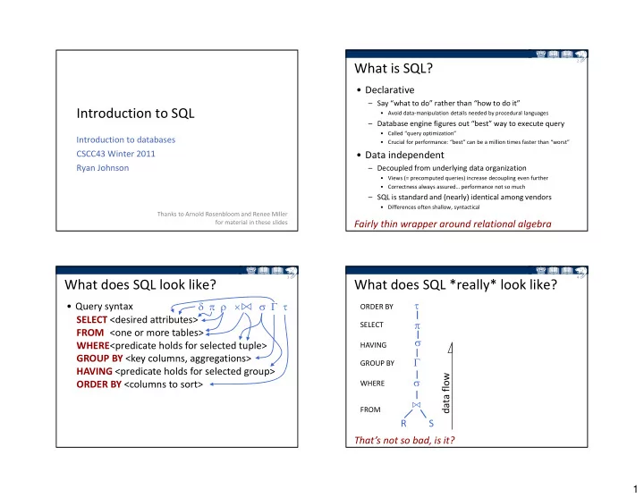
What does SQL look like?

Query syntax

SELECT <desired attributes> FROM <one or more tables> WHERE<predicate holds for selected tuple> GROUP BY <key columns, aggregations> HAVING <predicate holds for selected group> ORDER BY <columns to sort>  

4

What does SQL really look like?

FROM WHERE SELECT GROUP BY HAVING

  R S   

ORDER BY

data flow That’s not so bad, is it?

SLIDE 2

2

5

Other aspects of SQL

Updates, transactions

– Insert, delete, update rows – Transaction management – Consistency levels

“Active” logic

– Triggers and constraints – User‐defined functions, stored procedures

Data definition (sub)language (“DDL”)

– Manipulate database schema – Specify, alter physical data layout

We’ll come back to these later in the course

6

‘FROM’ clause

Identifies the tables (relations) to query

– Comma‐separated list

Optional: specify joins

– … but often use WHERE clause instead

Optional: rename table (“tuple variable”)

– Using the same table twice (else they’re ambiguous) – Nested queries (else they’re unnamed)

7

‘FROM’ clause – examples

Employees [AS] E

=> Table alias (most systems don’t require “AS” keyword)

Employees, Sales

=> Cartesian product

Employees E JOIN Sales S

=> Cartesian product (no join condition given!)

Employees E JOIN Sales S ON E.EID=S.EID

=> Equijoin

8

‘FROM’ clause – examples (cont)

Employees NATURAL JOIN Sales

=> Natural join (bug‐prone, use equijoin instead)

Employees E

LEFT JOIN Sales S ON E.EID=S.EID

=> Left join

Employees E1

JOIN Employees E2 ON E1.EID < E2.EID

=> Theta self‐join (what does it return?)

SLIDE 3

3

9

Gotcha: natural join in practice

Uses *all* same‐named attributes

– May be too many (self‐join => interesection => no‐op) – May be too few (almost‐same names => Cartesian product)

Implicit nature reduces readability

– Better to list explicitly all join conditions

Fragile under schema changes

– Nasty interaction of above two cases..

10

Gotcha: join selectivity

Consider tables R, S, T with T=Ø and this query:

SELECT R.x FROM R,S,T WHERE R.x=S.x OR R.x=T.x

Result contains no rows!

– Selection operates on pre‐joined tuples – R  S  T = R  S  Ø = Ø => No tuples for WHERE clause to work with! – Alternative: for loops assigning tuples to variables R, S, T => Empty relation => zero iterations => empty result

Workaround?

– Two coming up later

Moral of the story: WHERE cannot create tuples

11

Explicit join ordering

Use parentheses to group joins

– e.g. (A join B) join (C join D)

Special‐purpose feature

– Helps some (inferior) systems optimize better – Helps align schemas for natural join

Recommendation: avoid

– People are notoriously bad at optimizing things – Optimizer usually does what it wants anyway … but sometimes treats explicit ordering as a constraint

12

Scalar expressions in SQL

Literals, attributes, single‐valued relations
Boolean expressions

– Boolean T/F coerce to 1/0 in arithmetic expressions – Zero/non‐zero coerce to F/T in boolean expressions

Logical connectors: AND, OR, NOT
Conditionals

= != < > <= >= <> BETWEEN, [NOT] LIKE, IS [NOT] NULL, …

Operators: + ‐ * / % & | ^
Functions: math, string, date/time, etc. (more later)

Similar to expressions in C, python, etc.

SLIDE 4

4

13

‘SELECT’ clause

Identifies which attribute(s) query returns

– Comma‐separated list => Determines schema of query result

Optional: extended projection

– Compute arbitrary expressions – Usually based on selected attributes, but not always

Optional: rename attributes

– “Prettify” column names for output – Disambiguate (E1.name vs. E2.name)

Optional: specify groupings

– More on this later

Optional: duplicate elimination

– SELECT DISTINCT …

14

‘SELECT’ clause – examples

E.name

=> Vanilla projection

name

=> Implicit relation (error if R.name and S.name exist)

E.name [AS] ‘Employee name’

=> Prettified for output (like table renaming, ‘AS’ usually not required)

sum(S.value)

=> Grouping (compute sum)

sum(S.value)*0.13 ‘HST’

=> Computed value based on aggregate

123 ‘Magic number’

=> Filler column

*, E.*

=> Select all attributes, all attributes from E (no projection)

15

‘WHERE’ clause

Conditions which all returned tuples must meet

– Arbitrary boolean expression – Combine multiple expressions with AND/OR

Zero in on data of interest

– Specific people, dates, places, quantities – Things which do (or do not) correlate with other data

Often used instead of JOIN

– SELECT tables (Cartesian product, e.g. A, B) – Specify join condition (e.g. A.ID=B.ID) – Optimizers (usually) understand and do the right thing

16

‘WHERE’ clause – examples

S.date > ‘01‐Jan‐2010’

=> Simple tuple‐literal condition

E.EID = S.EID

=> Simple tuple‐tuple condition (equijoin)

E.EID = S.EID AND S.PID = P.PID

=> Conjunctive tuple‐tuple condition (three‐way equijoin)

S.value < 10 OR S.value > 10000

=> Disjunctive tuple‐literal condition

SLIDE 5

5

17

Pattern matching

Compare a string to a pattern

– <attribute> LIKE <pattern> – <attribute> NOT LIKE <pattern>

Pattern is a quoted string

% => “any string” _ => “any character”

To escape ‘%’ or ‘_’:

– LIKE ‘%x_%’ ESCAPE ‘x’ (replace ‘x’ with character of choice) => matches strings containing ‘_’

DBMS increasingly allow regular expressions

18

Pattern matching – examples

phone LIKE ‘%268‐_ _ _ _’

– phone numbers with exchange 268 – WARNING: spaces only shown for clarity

last_name LIKE ‘Jo%’

– Jobs, Jones, Johnson, Jorgensen, etc.

Dictionary.entry NOT LIKE ‘%est’

– Ignore ‘biggest’, ‘tallest’, ‘fastest’, ‘rest’, …

19

‘ORDER BY’ clause

Each query can sort by one or more attributes

– Refer to attributes by name or position in SELECT – Ascending (default) or descending (reverse) order – Equivalent to relational operator 

Definition of ‘sorted’ depends on data type

– Numbers use natural ordering – Date/time uses earlier‐first ordering – NULL values are not comparable, cluster at end or beginning

Strings are more complicated

– Intuitively, sort in “alphabetical order” – Problem: which alphabet? case sensitive? – Answer: user‐specified “collation order” – Default collation: case‐sensitive latin (ASCII) alphabet

String collation not covered in this class

20

‘ORDER BY’ clause – examples

E.name

=> Defaults to ascending order

E.name ASC

=> Explicitly ascending order

E.name DESC

=> Explicitly descending order

CarCount DESC, CarName ASC

=> Matches our car lot example from previous lecture

SELECT E.name … ORDER BY 1

=> Specify attribute’s position instead of its name

SLIDE 6

6

21

NULL values in SQL

Values allowed to be NULL

– Explicitly stored in relations – Result of outer joins

Possible meanings

– Not present (homeless man’s address) – Unknown (Julian Assange’s address)

Effect: “poison”

– Arithmetic: unknown value takes over expression – Conditionals: ternary logic (TRUE, FALSE, UNKNOWN) – Grouping: “not present”

22

Effect of NULL in expressions

Consider x having value NULL
Arithmetic: NaN

– x*0 NULL

Logic: “unknown”

– x OR FALSE NULL – x OR TRUE TRUE – x AND TRUE NULL – x AND FALSE FALSE – NOT x NULL

Ternary logic tricks: TRUE= 1 FALSE= 0 NULL= ½ AND = min(…) OR = max(…) NOT = 1‐x

Gotcha: x OR NOT x is unknown (why?)

23

Nested queries

Scary‐looking syntax, simple concept

– Treat one query’s output as input to another query – Inner schema determined by inner SELECT clause

Consider the expression tree

  R S vs.   S T   R

24

Nested queries – uses

Explicit join ordering

– FROM (A join B) is a (very simple) query to run first

Target of relation set operation

– Union, intersect, difference

One of several input relations for a larger query

– Appears in FROM clause – Usually joined with other tables (or other nested queries) => FROM A, (SELECT …) B WHERE … => Explicit join ordering is a degenerate case

SLIDE 7

7

25

Nested queries – more uses

Conditional relation expression

– Dynamic list for [NOT] IN operator => WHERE (E.id,S.name) IN (SELECT id,name FROM …) – Special [NOT] EXISTS operator => WHERE NOT EXISTS (SELECT * FROM …)

Scalar expression

– Must return single tuple (usually containing a single attribute) => 0.13*(SELECT sum(value) FROM Sales WHERE taxable) => S.value > (SELECT average(S.value) FROM Sales S)

26

Ways to represent nested queries

Nested subquery

– Arbitrary query in ‘FROM’ clause => Ad‐hoc (“one‐time”) usage

View

– Arbitrary query registered with database – Acts like a normal table, but contains “live” data => Good for frequent re‐use

Materialized view

– Query results stored as a normal table – DBMS updates it incrementally to keep data fresh => Good for complex queries or when data changes rarely

More on [materialized] views later in course…

27

Correlated subqueries

Two main types of nested query
Uncorrelated (subquery independent of tuples)

=> SELECT SR.name FROM SalesRep SR WHERE SR.ID IN (SELECT SRID FROM Complaints)

Correlated (inner depends on tuples)

=> SELECT SR.name FROM SalesRep SR WHERE EXISTS (SELECT ID FROM Complaints C WHERE SR.ID=C.SRID)

28

Correlated subqueries (cont)

Correlated = expensive

– System must re‐run subquery for each row

Often possible to convert correlated ‐>

uncorrelated

– Above examples are equivalent – Optimizers know this!

Often possible to flatten uncorrelated

=> SELECT SR.name FROM SalesRep SR, Complaints C WHERE SR.ID=C.SRID – Optimizers know this, too!

SLIDE 8

8

29

Union, intersection, and difference

Operations on pairs of subqueries
Expressed by the following forms

– (<subquery>) UNION [ALL] (<subquery>) – (<subquery>) INTERSECT [ALL] (<subquery>) – (<subquery>) EXCEPT [ALL] (<subquery>)

All three operators are set‐based

– Adding ‘ALL’ keyword forces bag semantics

Another solution to the join selectivity problem!

(SELECT R.x FROM R JOIN S ON R.x=S.x) UNION (SELECT R.x FROM R JOIN T ON R.x=T.x)

30

List comparisons: ANY, ALL, [NOT] IN

Compares a value against many others

– List of literals – Result of nested query

x op ANY (a, b, c)

= x op a OR x op b OR x op c

x op ALL (a, b, c)

= x op a AND x op b AND x op c

Op can be any comparator (>, <=, !=, etc.)

– x NOT IN (…) equivalent to x != ALL(…) – x IN (…) equivalent to x = ANY(…)

ANY is, ALL is (English usage often different!)

31

List comparisons – examples

SELECT * FROM Points p

WHERE 10 < ALL(p.x, p.y, p.z)

=> Select only points from bounding box near origin

SELECT * FROM Rectangles r

WHERE 10 > ANY(r.w, r.h)

=> Select rectangles with at least one large dimension

SELECT x FROM R

WHERE x IN (SELECT x FROM S) OR x IN (SELECT x FROM T)

=> Work around unwanted join selectivity

32

IN vs. join

R.x IN (…) is about tuples in R
R JOIN S on R.x=S.y is about R,S pairs
Ramification #1: bags

SELECT SR.name FROM SalesRep SR WHERE SR.ID IN (SELECT ID from CustomerComplaint) vs. SELECT SR.name FROM SalesRep SR JOIN CustomerComplaints CC ON SR.ID=CC.ID => Second version can return a name more than once

Ramification #2: join selectivity

SELECT x FROM R WHERE x IN (select x from S) OR x IN (select x from T) vs. SELECT R.x from R,S,T where R.x=S.x OR R.x=T.x => Second version fails if S or T is empty

Actually, both ramifications are equivalent

SLIDE 9

9

33

Operator: [NOT] EXISTS

Checks whether a subquery returned results
Example

– SELECT SR.name FROM SalesRep SR WHERE EXISTS (SELECT * FROM CustomerComplaints WHERE ID = SR.ID)

34

“SPJ” (select‐project‐join) queries

Most straightforward type
Operators available: 

– “Non‐blocking” (results trickle in as query runs) – Easiest to reason about – Easiest for system to optimize

Nesting OK

– Bonus: optimizer can often decorrelate, flatten query

Sorting, aggregation *not* OK!

– “Blocking” operators (query finishes before results show) – That includes 

Next up: aggregation

35

‘GROUP BY’ clause

Specifies grouping key of relational operator 

– Comma‐separated list of attributes (names or positions) which identify groups – Tuples agreeing in their grouping key are in same “group” – SELECT gives attributes to aggregate (and functions to use)

SQL specifies several aggregation functions

– COUNT, MIN, MAX, SUM, AVG, STD (standard deviation) – Some systems allow user‐defined aggregates

36

‘GROUP BY’ clause – gotchas

WHERE clause cannot reference aggregated

values

– Aggregates don’t “exist yet” when WHERE runs => Use HAVING clause instead

GROUP BY must list all non‐aggregate attributes

used in query

– Think projection => Some systems do this implicitly, others throw error

Grouping often (but not always!) sorts on

grouping key

– Depends on system and/or optimizer decisions => Use ORDER BY to be sure

SLIDE 10

10

37

‘GROUP BY’ clause – examples

SELECT SUM(value) FROM Sales

– No GROUP BY => no grouping key => all tuples in same group

SELECT EID, SUM(value) FROM Sales

– Error: non‐aggregate attribute missing from GROUP BY

SELECT EID, value FROM Sales GROUP BY 1,2

– Not an error – eliminates duplicates

SELECT SUM(value) FROM Sales GROUP BY EID

– Not an error, but rather useless: report per‐employee sales anonymously

38

‘GROUP BY’ clause – examples (cont)

SELECT EID, SUM(value)

FROM SALES GROUP BY EID

– Show total sales for each employee ID

SELECT EID, SUM(value), MAX(value)

FROM Sales GROUP BY 1

– Show total sales and largest sale for each employee ID

SELECT EID, COUNT(EID)

FROM Complaints GROUP BY EID

– Show how many complaints each salesperson triggered

39

Eliminating duplicates in aggregation

Use DISTINCT inside an aggregation

– SELECT EmpID, COUNT(DISTICT CustID) FROM CustomerComplaints GROUP BY 1 => Number of customers who complained about the employee => What if COUNT(CustID) >> COUNT(DISTINCT CustID)?

40

Effects of NULL on grouping

Short version: complicated

– Usually, “not present”

COUNT

– COUNT(R.) = 2 COUNT(R.x) = 1 – COUNT(S.) = 1 COUNT(S.x) = 0 – COUNT(T.*) = 0 COUNT(T.x) = 0

Other aggregations (e.g. MIN/MAX)

– MIN(R.x) = 1 MAX(R.x) = 1 – MIN(S.x) = NULL MAX(S.x) = NULL – MIN(T.x) = NULL MAX(T.x) = NULL

x  1 x x  R S T

This makes at least 3 ways COUNT is special

SLIDE 11

11

41

‘HAVING’ clause

Allows predicates on

aggregate values

– Groups which do not match the predicate are eliminated => HAVING is to groups what WHERE is to tuples

Order of execution

– WHERE is before GROUP BY => Aggregates not yet available when WHERE clause runs – GROUP BY is before HAVING => Scalar attributes still available

1