What is game theory? Study of interacting decision makers emphasis - - PDF document

SLIDE 1

S ystems

Analysis Laboratory

Helsinki University of Technology Session 11 - M. Järnefelt & T. Salminen Seminar on Microeconomics - Fall 1998 / 1

Session 11 - Chapter 15 Game Theory

Matias Järnefelt & Tuukka Salminen

S ystems

Analysis Laboratory

Helsinki University of Technology Session 11 - M. Järnefelt & T. Salminen Seminar on Microeconomics - Fall 1998 / 2

What is game theory?

Study of interacting decision makers – emphasis on cold-blooded, “rational” decision making. Generalisation of standard, one person decision theory – how should a rational expected utility maximiser behave in a situation in which his payoff depends on the choices of another expected utility maximiser? S ystems

Analysis Laboratory

Helsinki University of Technology Session 11 - M. Järnefelt & T. Salminen Seminar on Microeconomics - Fall 1998 / 3

Presentation outline

Description of a game, strategic form Simultaneous-move games

– Zero-sum & variable-sum games – Nash equilibrium – Repeated games

Sequential games

– Game tree ~ extensive form – Subgames – Information set

Bayes-Nash equilibrium (incomplete information)

S ystems

Analysis Laboratory

Helsinki University of Technology Session 11 - M. Järnefelt & T. Salminen Seminar on Microeconomics - Fall 1998 / 4

• Description of a game
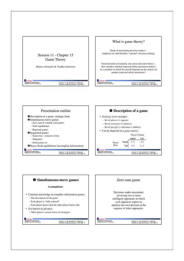
• Strategic form includes:

– Set of players (= agents) – Set of strategies (= choices) – Set of payoffs (= outcomes = utilities)

• Can be depicted in a game matrix:

Player Column Head Tail Head 1,-1

• 1,1

Player Row Tail

• 1,1

1,-1 S ystems

Analysis Laboratory

Helsinki University of Technology Session 11 - M. Järnefelt & T. Salminen Seminar on Microeconomics - Fall 1998 / 5

• Simultaneous-move games

Assumptions:

• Common knowledge in complete information games:

– The description of the game – Each player is “fully rational” – Each player knows that the other player knows this

• Not known in advance:

– Other player’s actual choice of strategies S ystems

Analysis Laboratory

Helsinki University of Technology Session 11 - M. Järnefelt & T. Salminen Seminar on Microeconomics - Fall 1998 / 6

Decisions under uncertainty involving two or more intelligent opponents in which each opponent aspires to

• ptimise his own decision at the

expense of other opponents.

Zero-sum game

SLIDE 2

S ystems

Analysis Laboratory

Helsinki University of Technology Session 11 - M. Järnefelt & T. Salminen Seminar on Microeconomics - Fall 1998 / 7

Player Column Head Tail Head 1

• 1

Player Row Tail

• 1

1

Zero-sum game

• Game of two players (Row & Column), where

payoffC = - payoffR

• Example: Matching pennies

S ystems

Analysis Laboratory

Helsinki University of Technology Session 11 - M. Järnefelt & T. Salminen Seminar on Microeconomics - Fall 1998 / 8

Variable-sum game

• Example: The Prisoner’s Dilemma

(two prisoners, duopoly, …)

• Aumann (1987) version:

Player Column Co-op Defect Co-op 3,3 0,4 Player Row Defect 4,0 1,1 S ystems

Analysis Laboratory

Helsinki University of Technology Session 11 - M. Järnefelt & T. Salminen Seminar on Microeconomics - Fall 1998 / 9

Example: Cournot duopoly

• Players: Two firms i=1, 2 producing a good at

zero cost facing inverse demand curve p(x)

• Strategy: Production level xi
• Payoff: Profit pi = p(x1 + x2)xi

S ystems

Analysis Laboratory

Helsinki University of Technology Session 11 - M. Järnefelt & T. Salminen Seminar on Microeconomics - Fall 1998 / 10

Example: Bertrand duopoly

• Similar to Prisoner’s Dilemma
• Players: Two firms i=1, 2 facing market

demand curve x(p)

• Strategy: Price pi of the good
• Payoff: π1(p1, p2) = p1 x(p1)

if p1 < p2 p1 x(p1)/2 if p1 = p2 if p1 > p2

S ystems

Analysis Laboratory

Helsinki University of Technology Session 11 - M. Järnefelt & T. Salminen Seminar on Microeconomics - Fall 1998 / 11

Pure & mixed strategies & beliefs

• R = set of pure strategies r available to Row
• Mixed strategy: probability of playing strategy r is pr
• Set of mixed strategies available to Row is the set of

all probability distributions (pr) over R

• Payoff to Row: ur(r, c)
• Row’s subjective probability distribution over

Column’s choices: (πc)

• Similarly: C, c, (pc), uc(r, c), (πr)

S ystems

Analysis Laboratory

Helsinki University of Technology Session 11 - M. Järnefelt & T. Salminen Seminar on Microeconomics - Fall 1998 / 12

Objectives

• Row’s objective:
• Column’s objective:

∑∑

π =

r c r c r p

c r u p

r

) , (

max

) (

∑∑

π =

c r c r c p

c r u p

c

) , (

max

) (

SLIDE 3

S ystems

Analysis Laboratory

Helsinki University of Technology Session 11 - M. Järnefelt & T. Salminen Seminar on Microeconomics - Fall 1998 / 13

Nash equilibrium

• A Nash equilibrium consists of probability beliefs

(πr , πc) over strategies, and probability of choosing strategies (pr , pc) such that:

1 The beliefs are correct: pr = πr and pc = πc ∀r, c ; and 2 Each player is choosing (pr) and (pc) so as to maximise his expected utility given his beliefs

• A Nash equilibrium in pure strategies is a pair (r*,c*)

such that

ur(r*, c*) ≥ ur(r, c*) ∀r and uc(r*, c*) ≥ uc(r*, c) ∀c S ystems

Analysis Laboratory

Helsinki University of Technology Session 11 - M. Järnefelt & T. Salminen Seminar on Microeconomics - Fall 1998 / 14

Nash Equilibrium

• Existence:

– Yes – with a finite number of agents and a finite number

• f pure strategies
• Uniqueness:

– Very unlikely in general – Further criteria to choose among Nash equilibria = refinements S ystems

Analysis Laboratory

Helsinki University of Technology Session 11 - M. Järnefelt & T. Salminen Seminar on Microeconomics - Fall 1998 / 15

Nash Equilibrium

Refinement:

• Dominant strategy:

r1, r2 ∈ R r1 strictly dominates r2 if ur(r1, c) > ur(r2, c) ∀c. r1 weakly dominates r2 if ur(r1, c) ≥ ur(r2, c) ∀c and ∃c’ so that ur(r1, c’) > ur(r2, c’)

• Dominant strategy equilibrium:

A choice of strategies by each player such that each strategy (weakly) dominates every other strategy available to that player

S ystems

Analysis Laboratory

Helsinki University of Technology Session 11 - M. Järnefelt & T. Salminen Seminar on Microeconomics - Fall 1998 / 16

Nash Equilibrium

If there is no dominant strategy equilibrium? Refinement:

• Elimination of strictly dominated strategies:

First eliminate all strategies that are strictly dominated and then calculate the Nash equilibria of the remaining game

• Example:

Player Column Left Right Top 2,2 0,2 Player Row Bottom 2,0 1,1 S ystems

Analysis Laboratory

Helsinki University of Technology Session 11 - M. Järnefelt & T. Salminen Seminar on Microeconomics - Fall 1998 / 17

About mixed strategies

• May be an unrealistic or the only sensible choice
• For any mixed strategy equilibrium, if one party

believes that the other player will play the equilibrium mixed strategy, then he is indifferent as to whether he plays his equilibrium mixed strategy,

• r any pure strategy that is part of the mixed strategy
• Reason: The expected utility function is linear in

probabilities

• Often mixed strategy probabilities

= population frequencies

S ystems

Analysis Laboratory

Helsinki University of Technology Session 11 - M. Järnefelt & T. Salminen Seminar on Microeconomics - Fall 1998 / 18

Repeated games

• A repeated game ≠ a repetition of a one-

shot game

• Each player can determine his choice at

some point as a function of the entire history of the game until that point

SLIDE 4

S ystems

Analysis Laboratory

Helsinki University of Technology Session 11 - M. Järnefelt & T. Salminen Seminar on Microeconomics - Fall 1998 / 19

Repeated games

• Example: Repeated Prisoner’s Dilemma
• Finite number of repetitions:

– Use of backwards induction ⇒ Nash Equilibrium = (Defect, Defect)

• Infinite number of repetitions:

– The payoffs are the discounted sums of the payoffs at each stage – Punishment strategy: Defect: payoff = 4 + 1/r, Co-operate: payoff = 3/r ⇒ Nash Equilibrium = (Co-operate, Co-operate) if r < ½ S ystems

Analysis Laboratory

Helsinki University of Technology Session 11 - M. Järnefelt & T. Salminen Seminar on Microeconomics - Fall 1998 / 20

Discussion on simultaneous-move games

The art of choosing a representation of the strategy choices of the game:

• Realism vs. simplicity
• What is relevant in modelling the set of strategies

used by the agents?

• Strategies should be difficult to change once the
• pponents behaviour is observed:

– One-shot / repeated vs. sequential game S ystems

Analysis Laboratory

Helsinki University of Technology Session 11 - M. Järnefelt & T. Salminen Seminar on Microeconomics - Fall 1998 / 21

Sequential games

• At least some of the choices are made sequentially
• One player may know the other player’s choice

before he has to make his own choice

• Games are described using the game tree: a diagram

that indicates the choices that each player can make at each point in time

S ystems

Analysis Laboratory

Helsinki University of Technology Session 11 - M. Järnefelt & T. Salminen Seminar on Microeconomics - Fall 1998 / 22

Game tree

Top Bottom Left Right Left Right ROW COL COL 1,9 1,9 0,0 2,1

The game tree The payoff matrix

Top Bottom Left Right COLUMN ROW 1,9 0,0 1,9 2,1

S ystems

Analysis Laboratory

Helsinki University of Technology Session 11 - M. Järnefelt & T. Salminen Seminar on Microeconomics - Fall 1998 / 23

Subgames and equilibria

• After a choice has been made, the strategies and

payoffs available make up a subgame

• The Nash equilibria can be calculated for each

possible subgame

• A strategy combination is a subgame perfect Nash

equilibrium if:

a) it is a Nash equilibrium for the entire game, and b) its relevant action rules are a Nash equilibrium for every subgame S ystems

Analysis Laboratory

Helsinki University of Technology Session 11 - M. Järnefelt & T. Salminen Seminar on Microeconomics - Fall 1998 / 24

Information set

The information set of an agent is the set of all nodes

• f the tree that cannot be differentiated by the agent.

Top Bottom Left Right Left Right ROW COL COL 1,9 1,9 0,0 2,1

SLIDE 5

S ystems

Analysis Laboratory

Helsinki University of Technology Session 11 - M. Järnefelt & T. Salminen Seminar on Microeconomics - Fall 1998 / 25

Example: A simple bargaining model

• Two players, A and B, have to divide $1
• They can negotiate at most three days, if they don’t

reach agreement, both get $0

• A offers day 1, B offers day 2, and A offers again

day 3

• A’s discount factor a, B’s multiplier b
• Method: backwards induction

S ystems

Analysis Laboratory

Helsinki University of Technology Session 11 - M. Järnefelt & T. Salminen Seminar on Microeconomics - Fall 1998 / 26

Day 3

• A can make a take-it-or-leave-it offer to B
• Thus, A offers B $0 (arbitrarily small amount): A

gets $1 and B gets $0

S ystems

Analysis Laboratory

Helsinki University of Technology Session 11 - M. Järnefelt & T. Salminen Seminar on Microeconomics - Fall 1998 / 27

Day 2

• B realises that A can guarantee himself $1 on the

next round by rejecting B’s offer

• Thus, B must offer A a payoff that has at least the

same present value for A as getting $1 tomorrow =a*$1

• B prefers 1-a now to zero next round
• The payoff to A=a and B=1-a

S ystems

Analysis Laboratory

Helsinki University of Technology Session 11 - M. Järnefelt & T. Salminen Seminar on Microeconomics - Fall 1998 / 28

Day 1

• A realises that B can get 1-a in the next round if he

rejects A’s offer

• Hence, A must offer B a payoff that has at least this

present value to B in order to avoid delay => A

• ffers B b(1-a) and game ends
• The final outcome: B gets b(1-a) and A gets 1-b(1-a).

S ystems

Analysis Laboratory

Helsinki University of Technology Session 11 - M. Järnefelt & T. Salminen Seminar on Microeconomics - Fall 1998 / 29

Illustration of the example

The case a=b<1

Ua Ub Day 1 budget constraint (xa+xb=1) b(1-a) 1-b(1-a) Day 2 budget constraint (xa+xb=a) Day 3 budget constraint (xa+xb=a*a) The final outcome

S ystems

Analysis Laboratory

Helsinki University of Technology Session 11 - M. Järnefelt & T. Salminen Seminar on Microeconomics - Fall 1998 / 30

Extension to infinite game

payoff to A b ab payoff to B b a ab = − − = − − 1 1 1 1 ( )

• Varian (p. 278): the subgame perfect

equilibrium division is:

• Note, if a=1 and b<1, then player A receives

the entire payoff and B gets nothing

SLIDE 6

S ystems

Analysis Laboratory

Helsinki University of Technology Session 11 - M. Järnefelt & T. Salminen Seminar on Microeconomics - Fall 1998 / 31

Repeated games and subgame perfection

• The idea of subgame perfection eliminates

Nash equilibria that are not credible, i.e. they are not in the interests of the players to carry

• E.g. punishing forever is not necessarily a

subgame perfect equilibrium

• Other strategies: Tit-for-Tat and the West

Point honor code

• Folk theorem: all distributions of utility in a

repeated one-shot game can be equilibria.

S ystems

Analysis Laboratory

Helsinki University of Technology Session 11 - M. Järnefelt & T. Salminen Seminar on Microeconomics - Fall 1998 / 32

Incomplete information

• The Nash equilibrium is not useful, if one agent does

not know the payoffs of the other agent

• Harsanyi (1967) approach subsumes all of the

uncertainty an agent has about another into a variable type

• Each agent defines a prior probability distribution
• ver the different types of agents

S ystems

Analysis Laboratory

Helsinki University of Technology Session 11 - M. Järnefelt & T. Salminen Seminar on Microeconomics - Fall 1998 / 33

Bayes-Nash equilibrium

• Each player knows that the other player is chosen

from a set of possible types, but does not know which type he belongs

• A Bayes-Nash equilibrium is a set of strategies for

each type of player that maximises the expected value of each type of player, given the strategies of the other players pursue

S ystems

Analysis Laboratory

Helsinki University of Technology Session 11 - M. Järnefelt & T. Salminen Seminar on Microeconomics - Fall 1998 / 34

Example: A sealed-bid auction

• Two bidders.
• Each know his own valuation, v, but neither knows

the others valuation => The type of the player refers to the valuation of the bidders

• Symmetric game: each player believes that the
• ther’s valuation is uniformly distributed between 0

and 1

S ystems

Analysis Laboratory

Helsinki University of Technology Session 11 - M. Järnefelt & T. Salminen Seminar on Microeconomics - Fall 1998 / 35

Functions

• A Bayes-Nash equilibrium to this game is a function

b(v), that describes the optimal bid, b, for a player of type v

• Let’s assume that b(v) is strictly increasing; higher

valuations lead to higher bids => There is a inverse function, V(b), that gives the valuation of someone bidding b

S ystems

Analysis Laboratory

Helsinki University of Technology Session 11 - M. Järnefelt & T. Salminen Seminar on Microeconomics - Fall 1998 / 36

Probabilities

• If a player bids b, his probability of winning is the

probability that the other bids less than b

• This equals the probability that the other player’s

valuation is less than V(b)

• v is uniformly distributed between 0 and 1 =>

P[V(other player)<V(b)]=V(b)

SLIDE 7

S ystems

Analysis Laboratory

Helsinki University of Technology Session 11 - M. Järnefelt & T. Salminen Seminar on Microeconomics - Fall 1998 / 37

Maximisation problem

• The expected payoff for player bidding b

when his valuation is v is:

(v-b)V(b)+0[1-V(b)]

• The optimal bid must maximise the above

expression, thus

(v-b)V’(b)-V(b)=0

• For each value of v, this equation determines

the optimal bid for the player as a function of v

S ystems

Analysis Laboratory

Helsinki University of Technology Session 11 - M. Järnefelt & T. Salminen Seminar on Microeconomics - Fall 1998 / 38

Solution

• The solution to the previous differential equation is

where C is a constant of integration

• When v=0, we must have b=0. Thus
• It follows, that C=0, and V(b)=2b or b=v/2.
• Thus, in Bayes-Nash equilibrium each player bids

half of their valuation V b b b C ( ) = + +

2

2 2 = + C S ystems

Analysis Laboratory

Helsinki University of Technology Session 11 - M. Järnefelt & T. Salminen Seminar on Microeconomics - Fall 1998 / 39

Discussion

• Art of eliminating “unreasonable” or “undesirable”

equilibria (too complex, etc.)

• Is Bayes-Nash equilibrium too involved?
• Different beliefs about the frequency of different

types of players leads to different optimal behaviour

S ystems

Analysis Laboratory

Helsinki University of Technology Session 11 - M. Järnefelt & T. Salminen Seminar on Microeconomics - Fall 1998 / 40

Additional literature

• Nalebuff, 1996. Co-opetition.
• Rasmusen, E., 1992. Games and informations - An

introduction to game theory.

• Ichiishi, T., 1991. Game theory and applications.
• Friedman J. W., 1986. Game theory with

applications to economics.