What is Cluster Analysis? Cluster: a collection of data objects - PowerPoint PPT Presentation

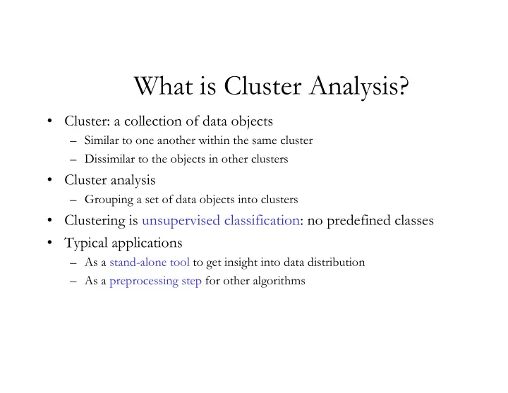
What is Cluster Analysis? • Cluster: a collection of data objects – Similar to one another within the same cluster – Dissimilar to the objects in other clusters • Cluster analysis – Grouping a set of data objects into clusters • Clustering is unsupervised classification: no predefined classes • Typical applications – As a stand-alone tool to get insight into data distribution – As a preprocessing step for other algorithms

Examples of Clustering Applications • Marketing: Help marketers discover distinct groups in their customer bases, and then use this knowledge to develop targeted marketing programs • Land use: Identification of areas of similar land use in an earth observation database • Insurance: Identifying groups of motor insurance policy holders with a high average claim cost • City-planning: Identifying groups of houses according to their house type, value, and geographical location • Earth-quake studies: Observed earth quake epicenters should be clustered along continent faults

What Is Good Clustering? • A good clustering method will produce high quality clusters with – high intra-class similarity – low inter-class similarity • The quality of a clustering result depends on both the similarity measure used by the method and its implementation. • The quality of a clustering method is also measured by its ability to discover some or all of the hidden patterns.

Measure the Quality of Clustering • Dissimilarity/Similarity metric: Similarity is expressed in terms of a distance function, which is typically metric: d ( i, j ) • There is a separate “ quality ” function that measures the “ goodness ” of a cluster. • The definitions of distance functions are usually very different for interval-scaled, boolean, categorical, and ordinal variables. • Weights should be associated with different variables based on applications and data semantics. • It is hard to define “ similar enough ” or “ good enough ” – the answer is typically highly subjective.

Spoofing of the Sum of Squares Error Criterion

Major Clustering Approaches • Partitioning algorithms: Construct various partitions and then evaluate them by some criterion • Hierarchy algorithms: Create a hierarchical decomposition of the set of data (or objects) using some criterion • Density-based: based on connectivity and density functions • Grid-based: based on a multiple-level granularity structure • Model-based: A model is hypothesized for each of the clusters and the idea is to find the best fit of that model to each other

Partitioning Algorithms: Basic Concept • Partitioning method: Construct a partition of a database D of n objects into a set of k clusters • Given a k , find a partition of k clusters that optimizes the chosen partitioning criterion – Global optimal: exhaustively enumerate all partitions – Heuristic methods: k-means and k-medoids algorithms – k-means (MacQueen ’ 67): Each cluster is represented by the center of the cluster – k-medoids or PAM (Partition around medoids) (Kaufman & Rousseeuw ’ 87): Each cluster is represented by one of the objects in the cluster

The K-Means Algorithm

The K-Means Clustering Method • Example 10 10 9 10 9 8 9 8 7 8 7 6 7 6 5 6 5 4 5 4 3 4 Update 3 Assign 2 3 2 the 1 each 2 1 cluster 0 1 objects 0 0 1 2 3 4 5 6 7 8 9 10 0 1 2 3 4 5 6 7 8 9 10 0 means to most 0 1 2 3 4 5 6 7 8 9 10 similar reassign reassign center 10 10 K=2 9 9 8 8 Arbitrarily choose K 7 7 object as initial 6 6 5 5 cluster center Update 4 4 the 3 3 2 2 cluster 1 1 means 0 0 0 1 2 3 4 5 6 7 8 9 10 0 1 2 3 4 5 6 7 8 9 10

Comments on the K-Means Method • Strength: Relatively efficient : O ( tkn ), where n is # objects, k is # clusters, and t is # iterations. Normally, k , t << n . • Comparing: PAM: O(k(n-k) 2 ), CLARA: O(ks 2 + k(n-k)) • Comment: Often terminates at a local optimum . The global optimum may be found using techniques such as: deterministic annealing and genetic algorithms • Weakness – Applicable only when mean is defined, then what about categorical data? – Need to specify k, the number of clusters, in advance – Unable to handle noisy data and outliers – Not suitable to discover clusters with non-convex shapes

The K - Medoids Clustering Method • Find representative objects, called medoids, in clusters • PAM (Partitioning Around Medoids, 1987) – starts from an initial set of medoids and iteratively replaces one of the medoids by one of the non-medoids if it improves the total distance of the resulting clustering – PAM works effectively for small data sets, but does not scale well for large data sets • CLARA (Kaufmann & Rousseeuw, 1990) • CLARANS (Ng & Han, 1994): Randomized sampling • Focusing + spatial data structure (Ester et al., 1995)

PAM (Partitioning Around Medoids) (1987) • PAM (Kaufman and Rousseeuw, 1987), built in Splus • Use real object to represent the cluster – Select k representative objects arbitrarily – For each pair of non-selected object h and selected object i , calculate the total swapping cost TC ih – For each pair of i and h , • If TC ih < 0, i is replaced by h • Then assign each non-selected object to the most similar representative object – repeat steps 2-3 until there is no change

PAM Clustering: Total swapping cost TC ih = � j C jih 10 10 j 9 9 t t 8 8 7 7 j 6 6 5 5 h i h 4 4 i 3 3 2 2 1 1 0 0 0 1 2 3 4 5 6 7 8 9 10 0 1 2 3 4 5 6 7 8 9 10 C jih = 0 C jih = d(j, h) - d(j, i) 10 10 i & t are 9 9 h the 8 8 j 7 7 current 6 6 i 5 i 5 mediods h j t 4 4 3 3 t 2 2 1 1 0 0 0 1 2 3 4 5 6 7 8 9 10 0 1 2 3 4 5 6 7 8 9 10 C jih = d(j, h) - d(j, t) C jih = d(j, t) - d(j, i)

What is the problem with PAM? • Pam is more robust than k-means in the presence of noise and outliers because a medoid is less influenced by outliers or other extreme values than a mean • Pam works efficiently for small data sets but does not scale well for large data sets. – O(k(n-k) 2 ) for each iteration where n is # of data,k is # of clusters è Sampling based method, CLARA(Clustering LARge Applications)

K-Means Clustering in R kmeans(x, centers, iter.max=10) x A numeric matrix of data, or an object that can be coerced to such a matrix (such as a numeric vector or a data frame with all numeric columns). centers Either the number of clusters or a set of initial cluster centers. If the first, a random set of rows in x are chosen as the initial centers. iter.max

Hartigan ’ s Rule When deciding on the number of clusters, Hartigan (1975, pp 90-91) suggests the following rough rule of thumb. If k is the result of k -means with k groups and k plus1 is the result with k +1 groups, then it is justifiable to add the extra group when: (sum(k$withinss)/sum(kplus1$withinss)-1)*(nrow(x)-k-1) is greater than 10.

Example Data Generation library(MASS) x1<-mvrnorm(100, mu=c(2,2), Sigma=matrix(c(1,0,0,1), 2)) x2<-mvrnorm(100, mu=c(-2,-2), Sigma=matrix(c(1,0,0,1), 2)) x<-matrix(nrow=200,ncol=2) x[1:100,]<-x1 x[101:200,]<-x2 pairs(x)

k -means Applied to our Data Set #Here we perform k=means clustering for a sequence of model #sizes x.km2<-kmeans(x,2) x.km3<-kmeans(x,3) x.km4<-kmeans(x,4) plot(x[,1],x[,2],type="n") text(x[,1],x[,2],labels=as.character(x.km2$cluster))

The 3 term k -means solution

The 4 term k -means Solution

Determination of the Number of Clusters Using the Hartigan Criteria > (sum(x.km3$withinss)/sum(x.km4$withinss)-1)*(200-3-1) [1] 23.08519 > (sum(x.km4$withinss)/sum(x.km5$withinss)-1)*(200-4-1) [1] 75.10246 > (sum(x.km5$withinss)/sum(x.km6$withinss)-1)*(200-5-1) [1] -6.553678 > plot(x[,1],x[,2],type="n") > text(x[,1],x[,2],labels=as.character(x.km5$cluster))

k =5 Solution

Hierarchical Clustering • Agglomerative versus divisive • Generic Agglomerative Algorithm: • Computing complexity O ( n 2 )

Distance Between Clusters

Height of the cross-bar shows the change in within-cluster SS Agglomerative

Hierarchical Clustering in R • Assuming that you have read your data into a matrix called data.mat then first you must compute the interpoint distance matrix using the dist function library(mva) data.dist<- dist(data.mat) • Next hierarchical clustering is accomplished with a call to hclust

hclust • It computes complete linkage clustering by default • Using the method= “ connected ” we obtain single linkage clustering • Using the method = “ average ” we obtain average clustering

plclust and cutree • plot is used to plot our dendrogram • cutree is used to examine the groups that are given at a given cut level