SLIDE 1
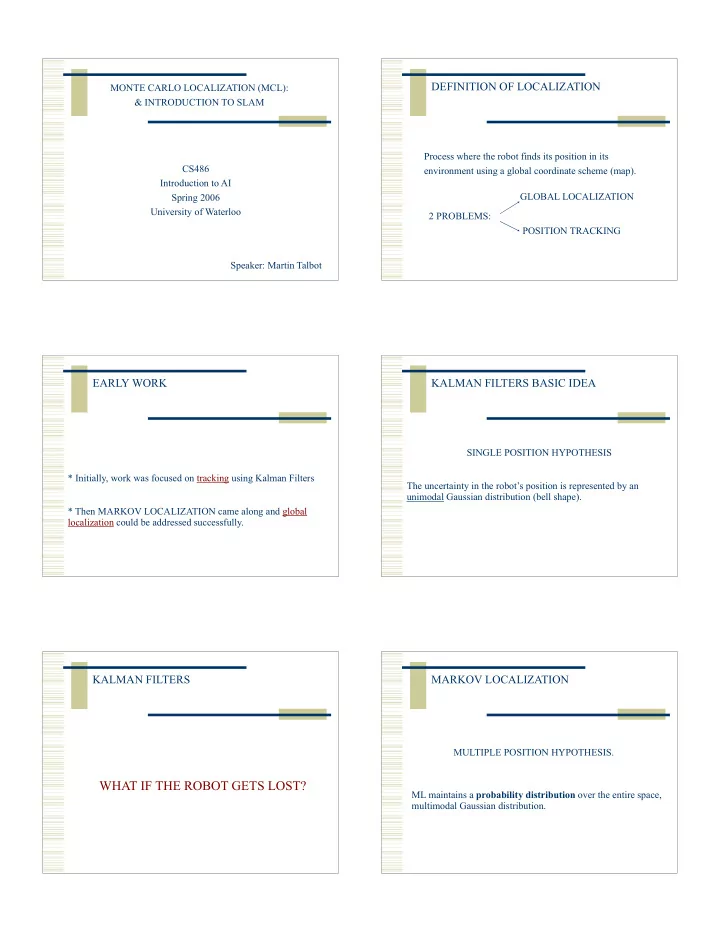
WHAT IF THE ROBOT GETS LOST? ML maintains a probability distribution - - PDF document

WHAT IF THE ROBOT GETS LOST? ML maintains a probability distribution - - PDF document
DEFINITION OF LOCALIZATION MONTE CARLO LOCALIZATION (MCL): & INTRODUCTION TO SLAM Process where the robot finds its position in its CS486 environment using a global coordinate scheme (map). Introduction to AI GLOBAL LOCALIZATION Spring
SLIDE 2
SLIDE 3
MATH BEHIND MARKOV LOCALIZATION
Bayes Filters address the problem of estimating the robot’s pose in its environment, where the pose is represented by a 2- dimensional Cartesian space with an angular direction. Example: pos(x,y, )
MATH BEHIND MARKOV LOCALIZATION
Bayes filters assume that the environment is Markov, that is past and future data are conditionally independent if one knows the current state
MATH BEHIND MARKOV LOCALIZATION
TWO TYPES OF MODEL: Perceptual data such as laser range measurements, sonar, camera is denoted by o (observed) Odometer data which carry information about robot’s motion is denoted by a (action)
MATH BEHIND MARKOV LOCALIZATION MATH BEHIND MARKOV LOCALIZATION MATH BEHIND MARKOV LOCALIZATION
MARKOV ASSUMPTION
SLIDE 4
MATH BEHIND MARKOV LOCALIZATION
We are working to obtain a recursive form…we integrate out xt-1 at time t-1
Using the Theorem of Total Probability
MATH BEHIND MARKOV LOCALIZATION
The Markov assumption also implies that given the knowledge
- f xt-1 and at-1, the state xt is conditionally independent of past
measurements up to time t-2
MATH BEHIND MARKOV LOCALIZATION
Using the definition of the belief Bel() we obtain a recursive estimation known as Bayes Filters. The top equation is of an incremental form.
MATH BEHIND MARKOV LOCALIZATION
Since both our motion model (a) and our perceptual model (o) are typically stationary (models don’t depend on specific time t) we can simplify the notation by using p(x’ | x, a) and p(o’|x’).
MATH BEHIND MARKOV LOCALIZATION
Bel(x’) = p(o’|x’) p(x’|x, a) Bel(x) dx
MONTE CARLO LOCALIZATION
Represent the belief Bel(x) by a set of discrete weighted samples. KEY IDEA:
SLIDE 5
MONTE CARLO LOCALIZATION
Bel(x) = {(l1,w1), (l2, w2), ….(lm, wm)} Where each li, 1 i m, represents a location (x,y,) Where each wi 0 is called the importance factor KEY IDEA:
MONTE CARLO LOCALIZATION
In global localization, the initial belief is a set of locations drawn according a uniform distribution, each sample has weight = 1/m.
MCL: THE ALGORITHM
The Recursive Update Is Realized in Three Steps
X’ = {(l1,w1)’, ….(lm, wm)’}
Step 1: Using importance sample from the weighted sample set representing ~ Bel(x) pick a sample xi: xi ~ Bel(x)
MCL: THE ALGORITHM
Step 2: Sample xi
’ ~ p(x’ | a, xi). Since xi and a together belong to a
distribution, we pick xi
t according to this distribution, the one that
has the highest probability is more likely to be picked.
MCL: THE ALGORITHM
Step 2: With xi
’ ~ p(x’ | xi, a) and xi ~ Bel(x) we compute
qt := xi
’ * xi note that this is: p(x’ | xi, a) * Bel(x)
MARKOV LOCALIZATION FORMULA!
We propose this distribution
MCL: THE ALGORITHM
SLIDE 6
The role of qt is to propose samples of the posterior distribution. This is not equivalent to the desired posterior.
MCL: THE ALGORITHM
Step 3: The importance factor w is obtained as the quotient of the target distribution and the proposal distribution.
MCL: THE ALGORITHM
p(x’ | xi, a) Bel(x) p(o’|xi
’) p(x’ | xi, a) Bel(x)
= p(o’|xi
’) wi
Target distribution Proposal distribution
MCL: THE ALGORITHM
Notice the proportionality between the quotient and wi ( is constant)
After m iterations, normalize w’
MCL: THE ALGORITHM ADAPTIVE SAMPLE SET SIZES
Use divergence of weight before and after sensing. Sampling is stopped when the sum of weights (action and
- bservation data) exceeds some threshold.
If action and observations are in tune together, each individual weight is large and the sample set remains small. If the opposite occurs, individual weights are small and the sample set is large. KEY IDEA:
ADAPTIVE SAMPLE SET SIZES
Global localization: ML 120 sec, MCL 3sec. Resolution 20 cm ~10 times more space than MCL with m=5000 samples
SLIDE 7