Variance - Making T (or ) Simpler Random Intercept Model: T = [ 00 - - PDF document

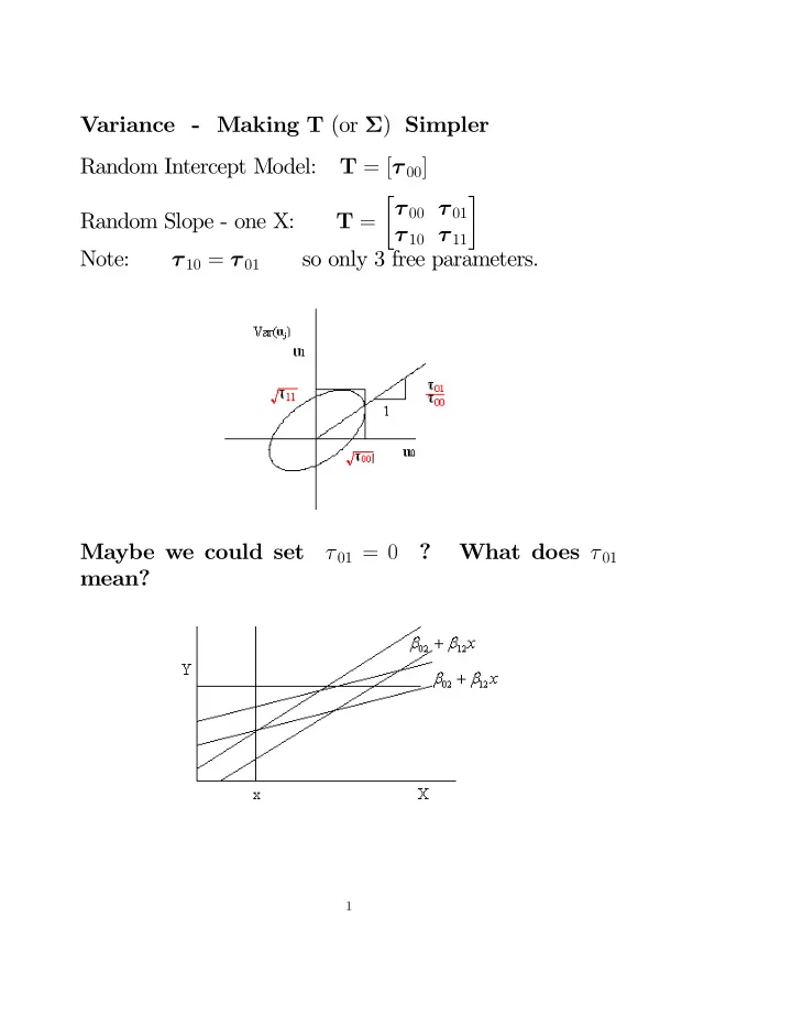
Variance - Making T (or Σ) Simpler Random Intercept Model: T = [τ 00] Random Slope - one X: T = τ 00 τ 01 τ 10 τ 11

• Note:

τ 10 = τ 01 so only 3 free parameters. Maybe we could set τ 01 = 0 ? What does τ 01 mean?

1

Consider variance of lines at X : V ar β0 β1

• =

τ 00 τ 01 τ 10 τ 11

• η = β0j + β1jX

= [1 X] β0j β1j

• V ar(η) = [1 X]

τ 00 τ 01 τ 10 τ 11 1 X

• = τ 00 + 2τ 01X + τ 11X2

quadratic in X If τ 11 > 0 then quadratic has a minimum at −τ 01 τ 11

• So forcing τ 01 = 0 is equivalent to assuming min SD at

X = 0

• This assumption is not invariant if we add a constant to

X

2

• Generally arbitrary and not warranted

Note: Centering for fixed part or random part or ran- dom part of model?

• With OLS, we can make: Cov (ˆ

β0, ˆ β1) = 0 by centering X at ¯ X

• With Mixed Models we can make:

Cov (β0j,β1j) = 0 by centering at −ˆ τ 01/ˆ τ 11 doesn’t justify imposing constraint. ** BUT often useful to improve convergence.

3

With 2 Random Slopes V ar   β0j β1j β2j   =   τ 00 τ 01 τ 02 τ 10 τ 11 τ 12 τ 20 τ 21 τ 22   uncond E(Y ) = γ00 + γ10X1 + γ20X2 E(Y ) ± SD is a bit harder but we can consider contours:

4

X2 X1 Contours of = SD

Guess shape of contours! Note: X1 X2

• min SD

= τ 11 τ 12 τ 21 τ 22 −1 τ 10 τ 20

• X2

X1 1

5

So, τ 12 = 0 <—> Cov (β1j,β2j) = 0 <—> Contour ellipse not tilted And, τ 22 = 0 => τ 21 = 0 => Contour horizontal So, in general:

• 1. Leave τ 01

τ 02 alone unless you recenter X1, X2 to

• X1

X2

• min SD

and set them to 0 for numerical reasons. (Caution: Iterate)

• 2. τ 12 = 0 might be a legitimate hypothesis.

Caution: low power in general so should use a C.I. if "accepting H0" (I get better results after centering in (1) but this is numerical)

6

Problem: How to set τ 12 = 0 ? Variance structures and parametrization. What do we know about:   τ 00 τ 01 τ 02 τ 11 τ 12 τ 22   Note: Only 6 parameters not 9 1. τ ii 0 2. ρij =

τ ij √τ ii√τ ij

Is this enough to be sure that T is a variance matrix? Answer: Yes for 2 x 2 but not enough for larger matrices Variance Matrix should be "positive-definite" — well... at least "non-negative definite"

7

Variance ellipses:

Positive Definite Positive Semi Definite Positive Semi Definite Positive Semi Definite degenerate ellipse 1 ± = ρ

8

What if not Non Negative Definite:

• r even nothing at all (actually: imaginary)!

Problem with Mixed Models: Keeping T non negative definite as estimation proceeds. One solution is "Cholesky parametrization" Idea: If T can be expressed in form T = ΛΛT for some matrix Λ then T is guaranteed to be a variance matrix Lower ∆ Cholesky [What SAS would do with FA0(3)]: Λ =   λ00 λ10 λ11 λ20 λ21 λ22   Note: 6 free parameters

9

T = ΛΛT =   λ00 λ10 λ11 λ20 λ21 λ22     λ00 λ10 λ20 λ11 λ21 λ22   =   λ2

00

λ00λ10 λ00λ20 λ2

10 + λ2 11 λ10λ20 + λ11λ21

λ2

20 + λ2 21 + λ2 22

  Note:

• Diagonal elements must be 0 (as expected)
• We can force first row of covariances to 0 by forcing

λ10 = λ20 = 0

• ther covariances τ 12 = λ11λ21 is not forced to 0.

BUT this is NOT what we really want.

• We can force first row of covariances to 0 by forcing

λ10 = λ20 = 0

• ther covariances τ 12 = λ11λ21 is not forced to 0.
• Forcing λ21 = 0 does not force τ 12 = 0

SAS Trick:

• Put intercept last in RANDOM statement.

Then you can use PARMS to force λ21 = 0 and τ 12 will be 0. T will be:

10

V ar   β1j β2j β0j   =   λ2

11

λ11λ21 λ11λ01 λ2

21 + λ2 22 λ21λ01 + λ22λ02

λ2

01 + λ2 02 + λ2 00

  So we can constrain τ 12 = 0 by constrainng λ21 = 0 In SAS RANDOM X1 X2 INTERCEPT / TYPE = FA0(3) SUB = ID G GC GCORR; PARMS (1) (0) (0.5) (0.021) (-0.03 (0.01) / HOLD = 2; Note: Fill in values from previous run or make good guess Note: S-Plus LME uses log Cholesky   eθ0 λ10 eθ1 λ20 λ21 eθ2   parameters: θ1, θ2, θ3, λ10, λ20, λ21 Which is an unconstrained parametrization of PD matrices. Default parametrization in SAS: TYPE = VC is diagonal

11

  τ 00 τ 11 τ 22   Which violates "τ ok" principle Some other SAS parametrizations TYPE = UN Unstructured - anything ... not necessarily a vanance matrix TYPE = AR (1)     1 ρ ρ2 ρ3 ρ 1 ρ ρ2 ρ2 ρ 1 ρ ρ3 ρ2 ρ 1     useful for for R (Σ) matrix for longitudinal data TYPE = UN (1) . . . See PROC MIXED p 2002 ff. Many of these will be more useful for longitudinal models.

• I would like to have Block Diagonal for variables other

than intercept and anything for cov with intercept, e.g:

12

— Consider:     τ 11 τ 12 τ 13 τ 10 τ 21 τ 22 τ 23 τ 20 τ 31 τ 32 τ 33 τ 30 τ 01 τ 02 τ 03 τ 00     — Would like:     τ 11 τ 12 τ 10 τ 21 τ 22 τ 20 τ 33 τ 30 τ 01 τ 02 τ 03 τ 00     — Can get this with Λ :     λ11 λ21 λ22 λ33 λ01 λ02 λ03 λ00     — Block diagonal structure in upper left square parti- tion of Λ is reproduced in T — So we can do this with PARMS by forcing upper-left elements of Λ to be 0

• Why this particular structure?

— If X1 , X2 are dummy variables for a 3-level cate- gorical variable it generally does not make sense to require τ 12 = 0 (not invariant w.r.t. recoding). But it does makes sense to ask whether the effect of the categorical variable is independent of X3

13

Note: that for PROC NLMIXED you can do Cholesky by

• hand. So might as well use log-Cholesky

14

Tests and C.I.’s for T (Σ) Wald, Wilks and Fisher OR - How far are we from the summit? Note: curvature of log-likelihood = "info"

• For τ ij

(i = j) we can test τ ij = 0 with a valid test

• More problematic for τ ii = 0 since τ ii can not be < 0
• If Ho :

τ ii = 0 and no other covariances are implied some advocate x p-value by 2.

• If we are also dropping covariances, we could use simu-

lation - but probably not in SAS

15

• Bates & Pinheiro throw up their hands and use regular p

taking comfort from fact that the error is "conservative"

• but NOT if you are going to accept Ho!!

16