[PPT] - Nearest neighbor classifier Information retrieval 8 ! Databases, PowerPoint Presentation

SLIDE 1

Subhransu Maji

29 January 2015

CMPSCI 689: Machine Learning

3 February 2015

Nearest neighbor classifier

Subhransu Maji (UMASS) CMPSCI 689 /37

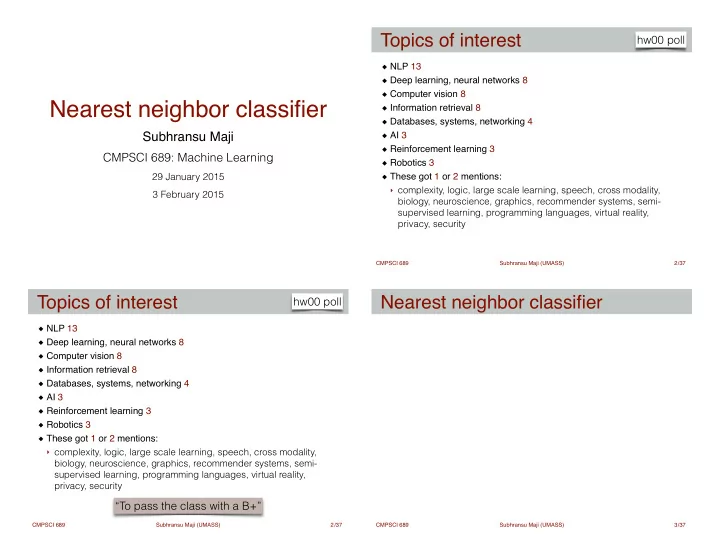
NLP 13! Deep learning, neural networks 8! Computer vision 8! Information retrieval 8! Databases, systems, networking 4! AI 3! Reinforcement learning 3! Robotics 3! These got 1 or 2 mentions:!

complexity, logic, large scale learning, speech, cross modality,

biology, neuroscience, graphics, recommender systems, semi- supervised learning, programming languages, virtual reality, privacy, security

Topics of interest

2

hw00 poll

Subhransu Maji (UMASS) CMPSCI 689 /37

NLP 13! Deep learning, neural networks 8! Computer vision 8! Information retrieval 8! Databases, systems, networking 4! AI 3! Reinforcement learning 3! Robotics 3! These got 1 or 2 mentions:!

complexity, logic, large scale learning, speech, cross modality,

biology, neuroscience, graphics, recommender systems, semi- supervised learning, programming languages, virtual reality, privacy, security

Topics of interest

2

“To pass the class with a B+” hw00 poll

Subhransu Maji (UMASS) CMPSCI 689 /37

Nearest neighbor classifier

3

SLIDE 2

Subhransu Maji (UMASS) CMPSCI 689 /37

Will Alice like AI?

Alice and James are similar and James likes AI. Hence, Alice must

also like AI.

Nearest neighbor classifier

3 Subhransu Maji (UMASS) CMPSCI 689 /37

Will Alice like AI?

Alice and James are similar and James likes AI. Hence, Alice must

also like AI. It is useful to think of data as feature vectors

Use Euclidean distance to measure similarity

Nearest neighbor classifier

3 Subhransu Maji (UMASS) CMPSCI 689 /37

Will Alice like AI?

Alice and James are similar and James likes AI. Hence, Alice must

also like AI. It is useful to think of data as feature vectors

Use Euclidean distance to measure similarity

Data to feature vectors

Nearest neighbor classifier

3 Subhransu Maji (UMASS) CMPSCI 689 /37

Will Alice like AI?

Alice and James are similar and James likes AI. Hence, Alice must

also like AI. It is useful to think of data as feature vectors

Use Euclidean distance to measure similarity

Data to feature vectors

Binary: e.g. AI? {no, yes}

➡ {0,1} ➡ or {-20, 2}

Nearest neighbor classifier

3

SLIDE 3

Subhransu Maji (UMASS) CMPSCI 689 /37

Will Alice like AI?

Alice and James are similar and James likes AI. Hence, Alice must

also like AI. It is useful to think of data as feature vectors

Use Euclidean distance to measure similarity

Data to feature vectors

Binary: e.g. AI? {no, yes}

➡ {0,1} ➡ or {-20, 2}

Nearest neighbor classifier

3

X

Subhransu Maji (UMASS) CMPSCI 689 /37

Will Alice like AI?

Alice and James are similar and James likes AI. Hence, Alice must

also like AI. It is useful to think of data as feature vectors

Use Euclidean distance to measure similarity

Data to feature vectors

Binary: e.g. AI? {no, yes}

➡ {0,1} ➡ or {-20, 2}

Nominal: e.g. color = {red, blue, green, yellow}

➡ {0,1}ⁿ ➡ or {0,1,2,3}

Nearest neighbor classifier

3

X

Subhransu Maji (UMASS) CMPSCI 689 /37

Will Alice like AI?

Alice and James are similar and James likes AI. Hence, Alice must

also like AI. It is useful to think of data as feature vectors

Use Euclidean distance to measure similarity

Data to feature vectors

Binary: e.g. AI? {no, yes}

➡ {0,1} ➡ or {-20, 2}

Nominal: e.g. color = {red, blue, green, yellow}

➡ {0,1}ⁿ ➡ or {0,1,2,3}

Nearest neighbor classifier

3

X X

Subhransu Maji (UMASS) CMPSCI 689 /37

Will Alice like AI?

Alice and James are similar and James likes AI. Hence, Alice must

also like AI. It is useful to think of data as feature vectors

Use Euclidean distance to measure similarity

Data to feature vectors

Binary: e.g. AI? {no, yes}

➡ {0,1} ➡ or {-20, 2}

Nominal: e.g. color = {red, blue, green, yellow}

➡ {0,1}ⁿ ➡ or {0,1,2,3}

Real valued: e.g. temperature

➡ copied ➡ or {low, medium, high}

Nearest neighbor classifier

3

X X

SLIDE 4

Subhransu Maji (UMASS) CMPSCI 689 /37

Training data is in the form of ! Fruit data:!

label: {apples, oranges, lemons}
attributes: {width, height}

Euclidean distance

Nearest neighbor classifier

4

(x1, y1), (x2, y2), . . . , (xn, yn)

height width

d(x1, x2) = sX

i

(x1,i − x2,i)2

Subhransu Maji (UMASS) CMPSCI 689 /37

Nearest neighbor classifier

5 Subhransu Maji (UMASS) CMPSCI 689 /37

Nearest neighbor classifier

5

test data (a, b) ?

Subhransu Maji (UMASS) CMPSCI 689 /37

Nearest neighbor classifier

5

test data (a, b) ?

SLIDE 5

Subhransu Maji (UMASS) CMPSCI 689 /37

Nearest neighbor classifier

5

test data (a, b) ?

Subhransu Maji (UMASS) CMPSCI 689 /37

Nearest neighbor classifier

5

test data (a, b) ? lemon

Subhransu Maji (UMASS) CMPSCI 689 /37

Nearest neighbor classifier

5

test data

Subhransu Maji (UMASS) CMPSCI 689 /37

Nearest neighbor classifier

5

test data (c, d) ?

SLIDE 6

Subhransu Maji (UMASS) CMPSCI 689 /37

Nearest neighbor classifier

5

test data (c, d) ?

Subhransu Maji (UMASS) CMPSCI 689 /37

Nearest neighbor classifier

5

test data (c, d) ?

Subhransu Maji (UMASS) CMPSCI 689 /37

Nearest neighbor classifier

5

test data (c, d) ? apple

Subhransu Maji (UMASS) CMPSCI 689 /37

k-Nearest neighbor classifier

6

utlier

SLIDE 7

Subhransu Maji (UMASS) CMPSCI 689 /37

k-Nearest neighbor classifier

6

What is the effect of k? Take majority vote among the k nearest neighbors

utlier

8

h > 8 yes lemon w > 7.3 no yes h > 7.8 yes orange no apple

SLIDE 9

Subhransu Maji (UMASS) CMPSCI 689 /37

Decision boundaries: DT

8

h > 8 no yes lemon w > 7.3 no yes h > 7.8 yes orange no apple

Subhransu Maji (UMASS) CMPSCI 689 /37

Decision boundaries: DT

8

h > 8 w > 6.6 no yes lemon w > 7.3 no yes h > 7.8 yes orange no apple

Subhransu Maji (UMASS) CMPSCI 689 /37

Decision boundaries: DT

8

h > 8 w > 6.6 no yes orange yes lemon w > 7.3 no yes h > 7.8 yes orange no apple

Subhransu Maji (UMASS) CMPSCI 689 /37

Decision boundaries: DT

8

h > 8 w > 6.6 no no yes orange yes lemon w > 7.3 no yes h > 7.8 yes orange no apple

SLIDE 10

Subhransu Maji (UMASS) CMPSCI 689 /37

Decision boundaries: DT

8

h > 8 w > 6.6 h > 6 no no

range

no yes lemon yes orange yes lemon w > 7.3 no yes h > 7.8 yes orange no apple

Subhransu Maji (UMASS) CMPSCI 689 /37

Decision boundaries: DT

8

h > 8 w > 6.6 h > 6 no no

range

no yes lemon yes orange yes lemon w > 7.3 no yes h > 7.8 yes orange no apple

The decision boundaries ! are axis aligned for DT

Subhransu Maji (UMASS) CMPSCI 689 /37

Choice of features!

We are assuming that all features are equally important
What happens if we scale one of the features by a factor of 100?

Choice of distance function!

Euclidean, cosine similarity (angle), Gaussian, etc …
Should the coordinates be independent?

Choice of k

Inductive bias of the kNN classifier

9 Subhransu Maji (UMASS) CMPSCI 689 /37

“Texture synthesis” [Efros & Leung, ICCV 99]

An example

10

SLIDE 11

Subhransu Maji (UMASS) CMPSCI 689 /37

“Texture synthesis” [Efros & Leung, ICCV 99]

An example

10 Subhransu Maji (UMASS) CMPSCI 689 /37

“Texture synthesis” [Efros & Leung, ICCV 99]

An example

10 Subhransu Maji (UMASS) CMPSCI 689 /37

What is ?
Find all the windows in the image that match the neighborhood
To synthesize x

➡ pick one matching window at random ➡ assign x to be the center pixel of that window

An exact match might not be present, so find the best matches using

Euclidean distance and randomly choose between them, preferring better matches with higher probability

An example: Synthesizing one pixel

11

p

input image synthesized image

Slide from Alyosha Efros, ICCV 1999

Subhransu Maji (UMASS) CMPSCI 689 /37

What is ?
Find all the windows in the image that match the neighborhood
To synthesize x

➡ pick one matching window at random ➡ assign x to be the center pixel of that window

An exact match might not be present, so find the best matches using

Euclidean distance and randomly choose between them, preferring better matches with higher probability

An example: Synthesizing one pixel

11

p

input image synthesized image

Slide from Alyosha Efros, ICCV 1999

SLIDE 12

Subhransu Maji (UMASS) CMPSCI 689 /37

What is ?
Find all the windows in the image that match the neighborhood
To synthesize x

➡ pick one matching window at random ➡ assign x to be the center pixel of that window

An exact match might not be present, so find the best matches using

Euclidean distance and randomly choose between them, preferring better matches with higher probability

An example: Synthesizing one pixel

11

p

input image synthesized image

Slide from Alyosha Efros, ICCV 1999

Subhransu Maji (UMASS) CMPSCI 689 /37

An example: Synthesis results

12

french canvas rafia weave

Slide from Alyosha Efros, ICCV 1999

Subhransu Maji (UMASS) CMPSCI 689 /37

white bread brick wall

An example: Synthesis results

13

Slide from Alyosha Efros, ICCV 1999

Subhransu Maji (UMASS) CMPSCI 689 /37

An example: Synthesis results

14

Slide from Alyosha Efros, ICCV 1999

SLIDE 13

Subhransu Maji (UMASS) CMPSCI 689 /37

Starting from the initial image, “grow” one pixel at a time!

Application: remove an object from the image

An example: Growing Texture

15

Slide from Alyosha Efros, ICCV 1999

Subhransu Maji (UMASS) CMPSCI 689 /37

Curse of dimensionality! Speed

Practical issues when using kNN

16 Subhransu Maji (UMASS) CMPSCI 689 /37

Curse of dimensionality! Speed

Practical issues when using kNN

17

10x10 #bins = How many neighborhoods are there? d = 2

Subhransu Maji (UMASS) CMPSCI 689 /37

Curse of dimensionality! Speed

Practical issues when using kNN

17

10x10 #bins = 10ᵈ d = 1000 #bins = Atoms in the universe ~ 10⁸⁰ How many neighborhoods are there? d = 2

SLIDE 14

Subhransu Maji (UMASS) CMPSCI 689 /37

Curse of dimensionality! Speed!

Time taken by kNN for N points of D dimensions

➡ time to compute distances: O(ND) ➡ time to find the k nearest neighbor

O(k N) : repeated minima
O(N log N) : sorting
O(N + k log N) : min heap
O(N + k log k) : fast median

➡ Total time is dominated by distance computation

We can be faster if we are willing to sacrifice exactness

SLIDE 15

Subhransu Maji (UMASS) CMPSCI 689 /37

Simplest idea is to cluster the data!

Class ! 3 clusters
Cluster ! mean of points
Label of a test is the label of

the nearest cluster mean Run time memory!

O(ND) O(CD)

➡ C << N

Approximate kNN

19

x

Subhransu Maji (UMASS) CMPSCI 689 /37

Simplest idea is to cluster the data!

Class ! 3 clusters
Cluster ! mean of points
Label of a test is the label of

the nearest cluster mean Run time memory!

O(ND) O(CD)

➡ C << N

Approximate kNN

19

x How do we cluster the data?

Subhransu Maji (UMASS) CMPSCI 689 /37

Given (x1, x2, …, xn), k-means clustering aims to partition the n observations into k (≤ n) sets S = {S1, S2, …, Sk} so as to minimize the within-cluster sum of squares.

!

In other words, its objective is to find:

Clustering using k-means

20

http://en.wikipedia.org/wiki/K-means_clustering

cluster center

Subhransu Maji (UMASS) CMPSCI 689 /37

Given (x1, x2, …, xn), k-means clustering aims to partition the n observations into k (≤ n) sets S = {S1, S2, …, Sk} so as to minimize the within-cluster sum of squares.

!

In other words, its objective is to find:

Clustering using k-means

20

http://en.wikipedia.org/wiki/K-means_clustering

Easy to compute μ given S and vice versa. cluster center

SLIDE 16

Subhransu Maji (UMASS) CMPSCI 689 /37

Initialize k centers by picking k points randomly! Repeat till convergence (or max iterations)!

Assign each point to the nearest center (assignment step)

! ! !

Estimate the mean of each group (update step)

! ! !

Simple and works well in practice!

Multiple initializations
Provably fast

Lloyd’s algorithm for k-means

21 Subhransu Maji (UMASS) CMPSCI 689 /37

K-means in action

http://en.wikipedia.org/wiki/K-d_tree

split at the median

SLIDE 18

Subhransu Maji (UMASS) CMPSCI 689 /37

k-d tree: O(log N) query time

Approximate kNN

23

http://en.wikipedia.org/wiki/K-d_tree

split at the median

Subhransu Maji (UMASS) CMPSCI 689 /37

k-d tree: O(log N) query time

Approximate kNN

23

http://en.wikipedia.org/wiki/K-d_tree

split at the median

Subhransu Maji (UMASS) CMPSCI 689 /37

k-d tree: O(log N) query time

Approximate kNN

23

http://en.wikipedia.org/wiki/K-d_tree

split at the median

Subhransu Maji (UMASS) CMPSCI 689 /37

k-d tree: O(log N) query time

Approximate kNN

23

http://en.wikipedia.org/wiki/K-d_tree

split at the median

SLIDE 19

Subhransu Maji (UMASS) CMPSCI 689 /37

k-d tree: O(log N) query time

Approximate kNN

23

Decision trees?

http://en.wikipedia.org/wiki/K-d_tree

w > w₁ h > h₁ w > w₂

yes yes yes no

… …

no no

split at the median

Subhransu Maji (UMASS) CMPSCI 689 /37

Very simple setup!

Training: none
Testing: find k nearest neighbors and take the majority class label

An example of a non-parametric classifier: the number of parameters of the classifier grow with the size of the training data Practical issues!

Curse of dimensionality: worst case dataset size grows O(nᵈ)
Speed: clustering (using k-means) and k-d trees as approximations

kNN is likely to be competitive when:!

the number of features are relatively small (< 20)
the distance metric is good
the dataset is large

Research questions:!

Learning a good metric
Testing speed: RP trees, locality sensitive hashing (LSH), ….

Summary of kNN

24 Subhransu Maji (UMASS) CMPSCI 689 /37

It may not be possible to get perfect classification on data!

Measurement noise: sensors may be inaccurate
Information gap: Sometimes we just don’t have enough information

to make accurate predictions

➡ e.g. Class ratings have high variance

Will students like AI? (70% yes, 30% no)

➡ e.g. Image is blurry

Not everything is learnable

25

3 or 7? 2 or 7? The best error you can get is called the Bayes error

/36

Lets do a bit of learning theory …

26

SLIDE 20

Subhransu Maji (UMASS) CMPSCI 689 /37

Bayes optimal classifier and error

27 Subhransu Maji (UMASS) CMPSCI 689 /37

Bayes optimal classifier and error

27

(x, y) ∼ D(x, y) : training data

Subhransu Maji (UMASS) CMPSCI 689 /37

Bayes optimal classifier and error

27

(x, y) ∼ D(x, y) : training data `(y, ˆ y): loss function

Subhransu Maji (UMASS) CMPSCI 689 /37

Bayes optimal classifier and error

27

(x, y) ∼ D(x, y) : training data `(y, ˆ y): loss function ✏(ˆ y) = E(x,y)∼ D [`(y, ˆ y)]: expected error of a predictor

SLIDE 21

Subhransu Maji (UMASS) CMPSCI 689 /37

Bayes optimal classifier and error

27

(x, y) ∼ D(x, y) : training data `(y, ˆ y): loss function ✏(ˆ y) = E(x,y)∼ D [`(y, ˆ y)]: expected error of a predictor ✏(x, ˆ y) = Ey∼ D(y;x) [`(y, ˆ y)]: expected error of a predictor at x

Subhransu Maji (UMASS) CMPSCI 689 /37

Bayes optimal classifier and error

27

(x, y) ∼ D(x, y) : training data `(y, ˆ y): loss function ✏(ˆ y) = E(x,y)∼ D [`(y, ˆ y)]: expected error of a predictor ✏(x, ˆ y) = Ey∼ D(y;x) [`(y, ˆ y)]: expected error of a predictor at x ✏∗(x) = ✏(x, y∗) y∗(x) = arg minˆ

y ✏(x, ˆ

y): Bayes optimal classifier : Bayes error

Subhransu Maji (UMASS) CMPSCI 689 /37

Bayes optimal classifier and error

27

(x, y) ∼ D(x, y) : training data `(y, ˆ y): loss function ✏(ˆ y) = E(x,y)∼ D [`(y, ˆ y)]: expected error of a predictor ✏(x, ˆ y) = Ey∼ D(y;x) [`(y, ˆ y)]: expected error of a predictor at x ✏∗(x) = ✏(x, y∗) y∗(x) = arg minˆ

y ✏(x, ˆ

y): Bayes optimal classifier : Bayes error `(y, ˆ y) = ⇢ 1 if y 6= ˆ y

therwise

(x, y) (xnn, ynn) Devroye, 1981 For any k ≥ 5, ✏∗ ≤ ✏k

nn ≤ ✏∗

1 + r 2 k ! Cover-Hart, 1967 ✏∗ ≤ ✏1

nn ≤ 2✏∗

✏1

nn(x) = P(y = 1, ynn = 0; x, xnn) + P(y = 0, ynn = 1; x, xnn)

= D(y = 1; x)D(ynn = 0; xnn) + D(y = 0; x)D(ynn = 1; xnn) = 2D(y = 1; x)D(y = 0; x) ≤ 2 min (D(y = 1; x), D(y = 0; x)) = 2✏∗(x) As n → ∞ D(ynn; xnn) → D(y; x)

/36

Machine learning solved?

29 Subhransu Maji (UMASS) CMPSCI 689 /37

kNN is nearly optimal when there is infinite training data!

Says nothing about the finite sample case
Note: not all classifiers are (nearly) optimal even with infinite data

Bayes error is a function of features (x)!

We can get better Bayes error if we choose different the features

➡ If we had color in addition to the width and height, we would be able

classify the fruits more accurately.

How do we understand the performance of learners for the finite sample case?!

Bias-variance decomposition

Not really …

30

SLIDE 23

Subhransu Maji (UMASS) CMPSCI 689 /37

Standard way to decompose squared loss

Bias-variance decomposition

31

`(y, ˆ y) = (y − ˆ y)2 ✏ ∼ N(0; 2) (x1, y1), (x2, y2), . . . , (xn, yn) → ˆ f(x) y = f(x) + ✏ ¯ f(x) = E ˆ f(x)

E ⇣ y − ˆ f(x) ⌘2 = E h f(x) − ¯ f(x) 2i + E h ( ˆ f

x) − ¯

f(x) 2i + σ2

bias² variance noise training algorithm true function noise expectation of the learned function expectation is over datasets

Subhransu Maji (UMASS) CMPSCI 689 /37

Example: curve fitting

32

y = f(x) + ✏ f(x) = sin(πx)

✏ = N(0, 2) σ = 0.1

figures from https://theclevermachine.wordpress.com/tag/estimator-variance/ Subhransu Maji (UMASS) CMPSCI 689 /37

Example: curve fitting

32

y = f(x) + ✏ f(x) = sin(πx)

✏ = N(0, 2)

gn(x) = θ0 + θ1x + θ2x2 + . . . + θnxn

σ = 0.1

figures from https://theclevermachine.wordpress.com/tag/estimator-variance/ Subhransu Maji (UMASS) CMPSCI 689 /37

Example: curve fitting

32

y = f(x) + ✏ f(x) = sin(πx)

✏ = N(0, 2)

gn(x) = θ0 + θ1x + θ2x2 + . . . + θnxn 50 samples

σ = 0.1

figures from https://theclevermachine.wordpress.com/tag/estimator-variance/

SLIDE 24

Subhransu Maji (UMASS) CMPSCI 689 /37

Example: curve fitting

33 figures from https://theclevermachine.wordpress.com/tag/estimator-variance/ Subhransu Maji (UMASS) CMPSCI 689 /37

Bias-variance decomposition proof

34

¯ f = E ˆ f y = f + ✏ ✏ ∼ N(0; 2)

E ⇣ y − ˆ f) ⌘2 = E ⇣ f + ✏ − ˆ f ⌘2 = E ⇣ f − ˆ f ⌘2 + 2 = E ⇣ f − ¯ f + ¯ f − ˆ f ⌘2 + 2 = E h f − ¯ f 2i + E ⇣ ¯ f − ˆ f ⌘2 + 2E h f − ¯ f ⇣ ¯ f − ˆ f ⌘i + 2 = E h f − ¯ f 2i + E ⇣ ¯ f − ˆ f ⌘2 + 2E h⇣ f ¯ f − f ˆ f − ¯ f ¯ f + ¯ f ˆ f ⌘i + 2 = E h f − ¯ f 2i + E ⇣ ¯ f − ˆ f ⌘2 + 2

f ¯

f − f ¯ f − ¯ f ¯ f + ¯ f ¯ f

+ 2

= E h f − ¯ f 2i + E ⇣ ¯ f − ˆ f ⌘2 + 2

Subhransu Maji (UMASS) CMPSCI 689 /37

Bias-variance decomposition proof

34

¯ f = E ˆ f y = f + ✏ ✏ ∼ N(0; 2) Similar decomposition can be obtained for the 0/1 loss

E ⇣ y − ˆ f) ⌘2 = E ⇣ f + ✏ − ˆ f ⌘2 = E ⇣ f − ˆ f ⌘2 + 2 = E ⇣ f − ¯ f + ¯ f − ˆ f ⌘2 + 2 = E h f − ¯ f 2i + E ⇣ ¯ f − ˆ f ⌘2 + 2E h f − ¯ f ⇣ ¯ f − ˆ f ⌘i + 2 = E h f − ¯ f 2i + E ⇣ ¯ f − ˆ f ⌘2 + 2E h⇣ f ¯ f − f ˆ f − ¯ f ¯ f + ¯ f ˆ f ⌘i + 2 = E h f − ¯ f 2i + E ⇣ ¯ f − ˆ f ⌘2 + 2

f ¯

f − f ¯ f − ¯ f ¯ f + ¯ f ¯ f

+ 2

= E h f − ¯ f 2i + E ⇣ ¯ f − ˆ f ⌘2 + 2

Subhransu Maji (UMASS) CMPSCI 689 /37

Bias-variance tradeoff for learners

35

E ⇣ y − ˆ f ⌘2 = E h f − ¯ f 2i + E ⇣ ˆ f − ¯ f ⌘2 + σ2

error = bias + variance + noise

bias degree of the polynomial

curve fitting with polynomials

variance depth of the tree bias variance

decision tree

bias variance k

kNN regression

SLIDE 25

Subhransu Maji (UMASS) CMPSCI 689 /37

kNN classifiers!

geometry, metric, decision boundaries
effect of k
practical issues

➡ curse of dimensionality ➡ speed: clustering using k-means, k-d trees

Theory!

Bayes optimality
kNN is nearly Bayes optimal as training dataset size goes to infinity
Bias-variance decomposition
Understanding overfitting and underfitting

Summary

36 Subhransu Maji (UMASS) CMPSCI 689 /37

The fruit classification dataset is from Iain Murray at University of Edinburgh — http://homepages.inf.ed.ac.uk/imurray2/teaching/

ranges_and_lemons/.!

The slides on texture synthesis are from Efros and Leung’s ICCV 2009 presentation.! Figures of the bias-variance tradeoff are from https:// theclevermachine.wordpress.com/tag/estimator-variance/.

Slides credit

37