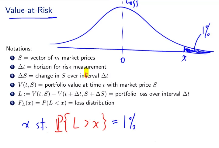
Value-at-Risk Notations: . S = vector of m market prices 1 . t = - - PowerPoint PPT Presentation

. .

Value-at-Risk

Notations: .

1

S = vector of m market prices .

2

∆t = horizon for risk measurement .

3

∆S = change in S over inverval ∆t .

4

V (t, S) = portfolio value at time t with market price S .

5

L := V (t, S) − V (t + ∆t, S + ∆S) = portfolio loss over interval ∆t .

6

FL(x) = P(L < x) = loss distribution

. .

Value-at-Risk

A few remarks: VaR is a measure of risk, but also reflects the sufficient capital to sustain large losses. The interval ∆t is typically quite short, e.g. 2 weeks for banks, as required by regulators. For fund management, the horizon is directly linked to the underlying assets (e.g. long/short term derivatives). For risk management purposes, it’s important to understand the sensitivies of VaR (or other risk measures) w.r.t time and underlying asset prices.

. .

Linear Portfolio under Multivariate Normal Distribution

The simplest approach to VaR is to consider the change in value ∆V = δT ∆S, for some vector of sensitivies δ. Assume ∆S ∼ N(0, ΣS) for some covariance matrix ΣS. Since L = −∆V ∼ N(0, σ2

L), where σ2 L = δT ΣSδ (a scalar).

E.g. the 99% VaR is 2.33σL (note: Φ(2.33) = 0.99). Here, we’re assuming a very small ∆t.

. .

Delta-Gamma Approximation

To capture nonlinear dependence of loss on underlying prices, we incorporate a 2nd-order sensitivity term. By Taylor expansion, we derive the delta-gamma (quadratic) approximation: ∆V ≈ ∂V ∂t ∆t + δT ∆S + 1 2∆ST Γ∆S, where δi = ∂V ∂Si , Γij = ∂2V ∂Si∂Sj are the 1st and 2nd derivatives of V . Again, we’re assuming a small ∆t. E.g. if V is the value of a European call on a stock S, then δ is the Delta and Γ is the Gamma of the option.

. .

MC Simulation of Loss Probabilities

In its simplest form, the MC simulation algorithm consists for the main steps:

.

1

Generate a vector of market moves ∆S (via Z) .

2

Compute portfolio loss −∆V . .

3

Estimate loss probability using 1 n

n

∑

i=1

1{Li>x} where Li is the ith sample loss.

The computation of portfolio value and thus its loss may be complicated and computationally expensive. The delta-gamma approximation can help accelerate the simulation. It also provides insights for variance reduction.

. .

Approximating Loss Distribution

We suppose that ∆S ∼ N(0, ΣS), and express it in terms of indep. normals ∆S = CZ, with Z ∼ N(0, I). For this to hold, we need to choose CCT = ΣS. The delta-gamma approximation of loss L = −∆V is L ≈ a − (CT δ)T Z − 1 2ZT (CT ΓC)Z, a = −∆t∂V ∂t

. .

Approximating Loss Distribution

To simplify the last term, we choose a C as follows: Obtain ˜ C from Cholesky factorization, s.t. ˜ C ˜ CT = ΣS. The symmetric matrix − 1

2 ˜

CT Γ ˜ C admits diagonalization: − 1

2 ˜

CT Γ ˜ C = UΛU T , where Λ is a diagonal matrix with filled with the eigenvalues λi, and U is an orthogonal matrix (UU T = I) of eigenvectors. Take C = ˜

• CU. Then, CCT = ˜

CUU T ˜ CT = ΣS. Also, − 1

2CT ΓC = 1 2U T ( ˜

CT Γ ˜ C)U = U T (UΛU T )U = Λ ← diagonal.

. .

Approximating Loss Distribution

As a result, setting b = −CT δ, we have L ≈ a + bT Z + ZT ΛZ = a +

m

∑

j=1

(bjZj + λjZ2

j ) ≡ Q.

Since the loss admits the approximation: L ≈ a +

m

∑

j=1

(bjZj + λjZ2

j ) ≡ Q,

the delta-gamma approximation yields the loss probability in terms of Q: P(L > x) ≈ P(Q > x).

. .

Importance Sampling

First, we look at the delta-gamma approximaion again: L ≈ a +

m

∑

j=1

(bjZj + λjZ2

j ) ≡ Q,

Here, Z’s are indep. standard normals, representing the sources of randomness. Since ∆S = CZ, or Z = C−1∆S → Z is linearly related to ∆S. Large losses would incur when

.

1

for j with bj > 0, Zj is large and positive; .

2

for j with bj < 0, Zj is large and negative; .

3

for j with λj > 0, Z2

j is large and positive.

What does this mean to importance sampling?

.

1

for j with bj > 0, assign a positive mean to Zj; .

2

for j with bj < 0, assign a negative mean to Zj; .

3

for j with λj > 0, increase the variance of Zj.

. .

Exponential Twisting

Recall Q = a + ∑m

j=1(bjZj + λjZ2 j ), which involves simulating standard

normals. For any mean vector µ and covariance matrix Σ, the likelihood ratio relating the density of N(µ, Σ) to N(0, I) is dP (0,I) dP (µ,Σ) = exp(− 1

2ZT Z)

|Σ|−0.5 exp ( − 1

2(Z − µ)T Σ−1(Z − µ)

). Hence, the loss probability can be expressed as P (0,I)  a +

m

∑

j=1

(bjZj + λjZ2

j ) > x

  = E(0,I) [ 1{Q>x} ] = E(µ,Σ) [ dP (0,I) dP (µ,Σ) 1{Q>x} ] .

. .

Loss Probability for a Portfolio of Options

Consider a portfolio of calls and puts on the same underlying S. Denote kc

i (resp. kp i ) be the no. of call (reps. put) with strike Ki and

maturity Ti. The portfolio value at time t is Wt =

n

∑

i=1

kc

i CBS(St; Ki, Ti)

• =:Ci(St)

+

m

∑

i=1

kp

i PBS(St; Ki, Ti)

• =:P i(St)

where CBS and PBS are the Black-Scholes price functions for calls and puts. We seek to estimate the loss probability P(Wt − Wt+∆t > x). Take t = 0, the initial wealth is W0 (constant) from the above equation.

. . 13 / 29

Applying Delta-Gamma Approximation

For small ∆t, assume ∆S ≈ S0(ˆ µ∆t + σ √ ∆tZ), with ˆ µ = µ − 0.5σ2. For each call option, the change in price is approximately ∆C ≈ ∂C ∂t ∆t + ∂C ∂S ∆S + 1 2 ∂2C ∂S2 ∆S2 = θc∆t + δcS0(ˆ µ∆t + σ √ ∆tZ) + γc 2 S2

0(ˆ

µ∆t + σ √ ∆tZ)2 ≈ bc

0 + bc 1Z + bc 2Z2,

where bc

0 = θc∆t + δcS0ˆ

µ∆t bc

1 = δcS0σ

√ ∆t bc

2 = γc

2 σ2S2

0∆t

The (call) Greeks θc, δc, and γc depend on strike and expiration date. Similar calculations yield the approximation ∆P ≈ bp

0 + bp 1Z + bp 2Z2, with

appropriate constants bp

0, bp 1, bp 2 involving the (put) Greeks θp, δp, and γp.

. .

Approximating Change in Portfolio Value

The portfolio loss is given by W0 − W∆t = −

n

∑

i=1

kc

i ∆Ci − m

∑

i=1

kp

i ∆P i

≈ −

n

∑

i=1

kc

i (bci 0 + bci 1 Z + bci 2 Z2) − m

∑

i=1

kp

i (bpi 0 + bpi 1 Z + bpi 2 Z2)

= h0 + h1Z + h2Z2, with constant coefficients h0, h1, h2.

. .

Exponential Twisting

Let f(z) be the standard normal pdf. Let κ(θ) be the moment generating function of h0 + h1Z + h2Z2: κ(θ) = E[eθ(h0+h1Z+h2Z2)]. Introduce a new function g(z) g(z) = eθ(h0+h1z+h2z2) κ(θ) · f(z) (1) = eθh0 √ 2πκ(θ) exp ( θh1z + (θh2 − 0.5)z2) . (2) Define ˆ σ2 = 1/(1 − 2θh2).

. .

Exponential Twisting

We re-write g by completing the square: g(z) = eθh0 √ 2πκ(θ) exp ( θh1z + (θh2 − 0.5)z2) = eθh0 √ 2πκ(θ) exp ( − 1 2ˆ σ2 (z2 − 2θh1 ˆ σ2z) ) = eθh0+0.5θ2h2

1ˆ

σ2

√ 2πκ(θ) exp ( − 1 2ˆ σ2 (z − θh1 ˆ σ2)2 ) = 1 √ 2πˆ σ exp ( − 1 2ˆ σ2 (z − θh1 ˆ σ2)2 ) ⇒ g ∼ N(θh1ˆ σ2, ˆ σ2) notice κ(θ) = ˆ σeθh0+0.5θ2h2

1ˆ

σ2.

In other words, g is indeed a normal pdf for any choice of θ.

. .

Simulation Algorithm

Generate N samples Vi’s from the distribution N(θh1ˆ σ2, ˆ σ2) of g. Calculate 1 N

N

∑

i=1

1{W0−W∆t(Vi)>x} f(Vi) g(Vi) where W∆t(Vi) is computed by the portfolio value based on the ith sample Vi.

. .

Loss Probability of Credit Portfolios

Suppose you have credit risk exposure on m different firms. Let Yi be the default indicator for firm i. Default probability of firm i: P(Yi = 1) = pi. When firm i default, a constant loss of ci is incurred. Portfolio loss: L = ∑m

i=1 ciYi.

Simulation is a useful way to estimate the loss distribution, or loss probability P(L > x)

• esp. for models with dependent defaults.

. .

Independent Defaults

Recall (loss) L = ∑m

i=1 ciYi, and (default prob.) P(Yi = 1) = pi.

If we assume defaults are independent, then loss L is a sum of indep. rv’s. The distribution of L is characterized by the moment generating function: E[eθL] = Πm

i=1E[eθciYi] = Πm i=1

( pieθci + (1 − pi) ) . For each firm i, we can define a new measure (distribution for Yi) via exponential twisting: dPθ dP = exp (θYi − ψ(θ)) , where ψi(θ) = log E[eθYi] = log ( pieθ + (1 − pi) ) . We can estimate each loss probability from the distribution Pθ: P(Yi = 1) = Eθ[ dP dPθ 1{Yi=1}].

. .

Independent Defaults

Recall (loss) L = ∑m

i=1 ciYi, and (default prob.) P(Yi = 1) = pi.

Differentiation of ψi(θ) = log E[eθYi] = log ( pieθ + (1 − pi) ) gives ψ′

i(θ) =

pieθ (pieθ + (1 − pi)), but this is in fact the probability of default under the measure Pθ because ψ′

i(θ) = E[eθYiYi]

E[eθYi] = E[eθYi−ψ(θ)Yi] = Eθ[Yi] = Pθ(Yi = 1) =: pi(θ).

. . 21 / 29

Independent Defaults

For exponential twisting to L (aggregate defaults), we define dPθ dP = exp (θL − ψL(θ)) , with ψL(θ) =

m

∑

i=1

ψi(ciθ) = Πm

i=1

eθciYi pieθci + (1 − pi). This expo. twisting is equivalent to twisting every ciYi. Under Pθ, we have pi(θ) = Pθ[Yi = 1] = ψ′

i(ciθ) =

pieciθ (pieciθ + (1 − pi)). We rearrange to get the ratio: pi(θ) 1 − pi(θ) = ( pi 1 − pi ) eθci. This shows that taking θ > 0 increases the default probability ratio for every firm, esp. for those with larger exposure ci.

. .

Dependent Defaults

We now incorporate dependence among defaults. For each firm i, we define xi = Φ−1(1 − pi), which means P(Xi > xi) = pi, for Xi ∼ N(0, 1). Construct default indicators by Yi = 1{Xi>xi}, i = 1, . . . , m. To introduce dependence, we link the rv’s Xi by X = AZ + Bϵ, where A is a m × k matrix, Z ∼ N(0, Ik) independent of ϵ ∼ N(0, Im), B is a diagonal matrix. Covariance matrix of X is C := AAT + B2. Choose (diagonal) entries of B s.t. diagonal entries of C are all 1 ⇒ X are standard normals.

. .

Conditional Default Probabilities

Recall: X = AZ + Bϵ. We can interpret Z as the common factors driving defaults, whereas ϵ are the firm specific factors. Conditioned on Z, the vector X is normally distributed with mean vector AZ (Z known after conditioning), and diagonal covariance matrix B2. Therefore, the conditional default probability for firm i is ˜ pi(Z) = P(Yi = 1|Z) = P(Xi > xi|Z) = 1 − Φ (xi − aiZ bi ) , (3) where ai is the ith row of A, and bi the ith element on the diag. of B. Hence, given Z, Xi and thus Yi are independent.

. .

Conditional Default Probabilities

Suppose: Let Xi = √ρZ + √ 1 − ρϵi, with IID N(0, 1) Z and ϵi’s. Let Yi = 1{Xi>x}; L = ∑

i Yi.

Note that L is just the number of defaults from m firms with conditional default probability ˜ p(Z) (same for all firms). Given Z = z, the defaults are independent with probability ˜ p(z). Therefore, the conditional distribution of L given Z = z is binomial: P(L = ℓ | Z = z) = (m ℓ ) ˜ p(z)ℓ(1 − ˜ p(z))m−ℓ. The unconditional probability is found from integration: P(L = ℓ) = ∫

R

(m ℓ ) ˜ p(z)ℓ(1 − ˜ p(z))m−ℓfZ(z)dz, where fZ is the pdf of Z. In other words, we just average the binomial distributions over possible values

• f Z weighted by its density function.

. .

Homogeneous Large Portfolio Approximation

We exploit that the no. of firms m is large to obtain a final approximation. Let Xi = √ρZ + √ 1 − ρϵi, with IID N(0, 1) Z and ϵi’s. Let Y = L/m be the loss fraction. Then, for y ∈ [0, 1], P(Y ≤ y) = ∫

R

P( L m ≤ y | Z = z)fZ(z)dz. We use the fact that, given Z = z, L is the sum of m (conditionally) independent Bernoulli rv’s with parameter ˜ p(z). By the law of large numbers, the long-run average L

m converges to the mean

• f the Bernoulli rv, i.e. ˜

p(z). Consequently, we have L m → ˜ p(z), and P( L m ≤ y | Z = z) → 1{˜

p(z)≤y}.

. .

Homogeneous Large Portfolio Approximation

Recall: all p ≡ pi, x ≡ xi = Φ−1(1 − p), ˜ p(z) = 1 − Φ( x−√ρz

√1−ρ ).

LLN gives the approximate distribution of loss fraction: P(Y ≤ y) ≈ ∫

R

1{˜

p(z)≤y}fZ(z)dz = P(˜

p(Z) ≤ y) = P ( 1 − y ≤ Φ (x − √ρZ √1 − ρ )) = P (x − √1 − ρΦ−1(1 − y) √ρ ≥ Z ) = Φ (x − √1 − ρΦ−1(1 − y) √ρ ) = Φ (Φ−1(1 − p) − √1 − ρΦ−1(1 − y) √ρ ) . That is, when no. of firms m is very large, the loss probability is approximated analytically, using the inputs p

. .

Conditional Exponential Twisting

Recall: X = AZ + Bϵ; Yi = 1{Xi>xi}; L = ∑

i ciYi.

The conditional distribution of L given Z is determined as in the independent case but with ˜ pi instead of pi. Define the cumulant generating function for L given Z ψL|Z(θ) = log E[eθL|Z] =

m

∑

i=1

log ( ˜ pieθci + (1 − ˜ pi) ) . Define the exponential twisting for L given Z by dPθ dP

• Z

:= exp(θL − ψL|Z(θ)). Again, choose θx s.t. ψ′

L|Z(θx) = x.

In turn, this gives the conditional probability under Pθ: ˜ pi(θx) := Pθx(Yi = 1|Z) = ˜ pieciθx (˜ pieciθx + (1 − ˜ pi)). (4)

. .

Simulation Algorithm for Credit Losses

Here’s a summary of the simulation procedure: Generate Z ∼ N(0, Ik). Compute ˜ pi from (3). Solve ψ′(θx) = x for θx (set it to 0 if negative, possible if ψ′

L|Z(0) > x).

Compute ˜ pi(θx) as in (4). Simulate Yi with probability ˜ pi(θx) that Yi = 1, and probability 1 − ˜ pi(θx) that Yi = 0. Sum up to get the loss L = c1Y1 + · · · + cmYm, and return the estimator e−θxL+ψL|Z(θx)1{L>x}.

. .

Importance Sampling for Z

Instead of generating Z ∼ N(0, I), we can apply importance sampling to introduce a non-zero mean to Z. For instance, we can multiply the estimator by the likelihood ratio: exp(− 1

2ZT Z)

exp ( − 1

2(Z − µ)T (Z − µ)

) = exp ( −µT Z + 1 2µT µ ) . As a result, we will sample Z from the new distribution N(µ, Ik), and apply the estimator: exp ( −µT Z + 1 2µT µ − θxL + ψL|Z(θx) ) 1{L>x}.