Using Math and Computing to Model Supernovae Andy Nonaka Lawrence - - PowerPoint PPT Presentation

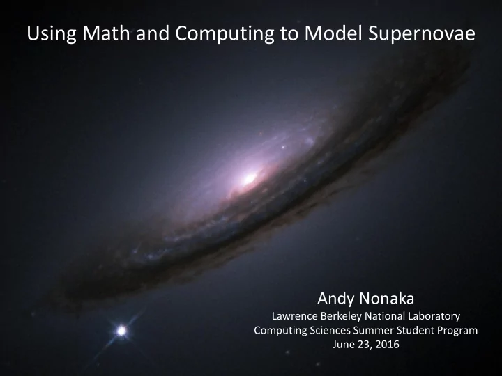
Using Math and Computing to Model Supernovae

Andy Nonaka

Lawrence Berkeley National Laboratory Computing Sciences Summer Student Program June 23, 2016

Galaxy NGC 4526 imaged by the Hubble Space Telescope (www.nasa.gov) 60 million light years away SN1994D (Type Ia supernova) The supernova is as bright as the host galaxy!

• Why should we care?
• Using modern telescopes, Type Ia supernova light curves

can now be observed several hundred times per year.

– Spectra indicate that oxygen and calcium are present early, where as nickel, cobalt, and iron are present later.

Type Ia Supernovae are Distance Indicators

• By observing Type Ia supernovae at known, nearby distances,

scientists have established a width-luminosity relationship; wider = brighter.

• Theory: by observing the peak luminosity and decay rate, we

can determine the distance to a host galaxy.

– Particularly useful for mapping distant galaxies since they are so bright!

Type Ia Supernovae are Speed Indicators

• Due to the observed redshift, we know

the speed at which the host galaxy is moving away from us.

– Led to discovery of the acceleration of the expansion of the universe in 1998 – 2011 Physics Nobel Prize (Perlmutter, LBNL)

• Problem: We don’t know how well the

width-luminosity relationship holds for distant Type Ia supernovae.

– Farther away = earlier in the life of the universe – Composition of stars was different back then… – Not even sure if accepted models properly describe nearby events…

Studying Type Ia Supernovae

• We study this problem using math and computing

– Develop mathematical models/equations describing stellar evolution and explosions – Develop numerical methods (algorithms) to solve these equations – Use supercomputers (10,000 – 100,000 CPUs) such as edison at NERSC.

• Requires expertise in applied math and computer

science.

• Requires expertise in astrophysics (collaborate with

experts in the field).

The Phases of Type Ia Supernovae: Single Degenerate Model

A white dwarf accretes matter from a binary companion over millions

• f years.

Smoldering phase characterized by subsonic convection and gradual temperature rise lasts hundreds of years. Flame (possibly) transitions to a detonation, causing the star to explode within two seconds. The resulting event is visible from Earth for weeks to months.

• D. A. Hardy & PPARC

Haitao Ma, UCSC SN 1994D (High-Z SN Search team)

Computing the Explosion Phase

• Over the past decade, many have performed studies
• f the explosion phase using supercomputers.

– Governed by well-understood (both theoretically and algorithmically) fluid dynamics equations. – A supercomputer can model this system in a few days or weeks, depending on spatial resolution.

Haitao Ma, UCSC

Our CASTRO code is one of many publicly available codes capable of modeling such explosions.

Governing Equations

• Equations describing a compressible, reacting fluid/gas:

u

Xk _ !k E ½ H

density mass fraction of species “k” reaction rate of species “k” velocity total energy per unit mass energy release due to reactions

p

pressure

g

gravity conservation of mass conservation of momentum conservation of energy

Basic Solution Methodology

• Equations describing a compressible, reacting fluid/gas:
• Finite volume approach.

– Divide problem into grid cells – Advance solution incrementally

• ver many time steps, Δt, until

final time achieved

conservation of mass conservation of momentum conservation of energy

Computing the Explosion Phase

Haitao Ma, UCSC

A major problem are the initial conditions, which have been based on “guesses”. What is the initial state of the star? Where are the first flames? How many ignition points are there?

The Phases of Type Ia Supernovae: Single Degenerate Model

A white dwarf accretes matter from a binary companion over millions

• f years.

Smoldering phase characterized by subsonic convection and gradual temperature rise lasts hundreds of years. Flame (possibly) transitions to a detonation, causing the star to explode within two seconds. The resulting event is visible from Earth for weeks to months.

• D. A. Hardy & PPARC

Haitao Ma, UCSC SN 1994D (High-Z SN Search team)

Computing the Convective Phase

• We would like to simulate the last few hours of

smoldering preceding the explosion to obtain initial conditions for CASTRO.

• Problem: It takes weeks on a supercomputer to

simulate 2 seconds of real-time. How do we simulate hours?

Governing Equations

• Compressible, reacting fluid equations:

conservation of mass conservation of momentum conservation of energy

• These equations describe 3 things:

– Motion of the fluid – Nuclear reactions (burning) – Sound waves

Smoldering Phase vs. Explosive Phase

• How is the smoldering phase different from the

explosion phase?

– “Low Mach Number” flow - fluid speed small compared to sound speed (~1%) – Sound waves carry little energy and have minimal impact

• n the overall solution
• “Ignoring” them doesn’t significantly affect the solution.
• We have derived a new equation set that ignores the

effect of sound waves, yet retains all the remaining physics, and is much more computationally efficient.

Low Mach Number Equation Set

• Derive new equations/model using low Mach number

asymptotics

– Mach number: M = U/c – Looks similar to the standard equations of compressible flow, but sound waves have been analytically removed

• Enables time steps constrained by the fluid velocity CFL, not the

sound speed CFL:

• Low Mach time step is a factor of 1/M larger than a compressible

time step, enabling longer simulations!

¢tcompressible < ¢x juj + c ¢tlowMach < ¢x juj

Computational Efficiency

• In our white dwarf simulations, the peak Mach

number varies from 0.01 – 0.05.

– Net result: the low Mach number time step is a factor of 70 greater than a compressible time step – However, the low Mach number equation set is more complex and takes approximately 2.5 times longer advance a single time step. – Thus, to advance the solution to the final time, MAESTRO is a factor of (70 / 2.5) ≈ 28 more efficient than a compressible algorithm, given the same number of computational resources for this problem. – Now we can simulate roughly 1 minute of the smoldering phase, but we are still looking to simulate several hours.

Adaptive Mesh Refinement

• For the full star problem, we need to consider our

refinement criteria

– Burning occurs near core, driving flow in the inner-convective region of the star. – We expect ignition point(s) to be near the center of the star

• Incorporate AMR using

established techniques

– Advance each level independently and synchronize solution between levels to maintain conservation

Adaptive Mesh Refinement

• 5763 (8.7 km)

– 1728 · 483 grids – 191 Million Cells 5000 km

Adaptive Mesh Refinement

• 5763 (8.7 km)

– 1728 · 483 grids – 191 Million Cells 5000 km Edge of Star Convective Zone Boundary

Adaptive Mesh Refinement

• 5763 (8.7 km)

– 1728 · 483 grids – 191 Million Cells

Adaptive Mesh Refinement

• 5763 (8.7 km)

– 1728 · 483 grids – 191 million cells

• 11523 (4.3 km)

– 1684 grids – 148 million cells – 9.7% of domain

• 23043 (2.2 km)

– 3604 grids – 664 million cells – 5.4% of domain

Adaptive Mesh Refinement

• A 23043 simulation

with no AMR would contain 12.2 billion cells.

• Our simulation

contains a total of 1.0 billion cells, requiring a factor of 12 less work.

5000 km

Adaptive Mesh Refinement

• In practice, we run

most of the simulation using the coarsest resolution only and add AMR in the last few minutes as the star approaches ignition.

– Allows us another factor of 20 speedup 5000 km

Parallelization Strategy

• Hybrid MPI/OpenMP approach to parallelization.

– Nodes assigned to grids, threads spawned on cores to work on grids

• We are able to efficiently run our codes on 100,000+

processors using this approach.

node

core core core core core core core core core core core core

node

core core core core core core core core core core core core

node

core core core core core core core core core core core core OpenMP Threads MPI Communication

White Dwarf Convection: Initial Conditions

Edge of Star density = 10-4 g/cc Center of Star density = 2.6 x 109 g/cc Temperature = 6.25 x 108 K 5000 km

• Initial conditions

– 1D model model mapped

• nto Cartesian grid

– Random velocity perturbation added to prevent initial nuclear runaway – Use 10K cores for 40 days (10 million CPU hours) to run effective 23043 resolution (2.2km zones) to ignition

White Dwarf Convection: Ignition

• Convective flow pattern

a few minutes preceding ignition

– Inner 1000 km3 of star – Effective 23043 resolution (2.2km) with 3 total levels of refinement – Red / Blue = outward / inward radial velocity – Yellow / Green = contours of increasing burning rate

• Red / Blue = outward / inward radial velocity
• Yellow / Green = contours of increasing burning rate

t = 15 minutes t = 50 minutes t = 80 minutes t = 115 minutes t = 150 minutes t ≈ 165 minutes (ignition)

White Dwarf Convection: Ignition

• Same data from the

previous simulation

• 2D slice of temperature

profile a few minutes preceding ignition

White Dwarf Convection: Long-Time Behavior

• Maximum temperature and Mach number vs. time

WD Convection: Ignition

• Examining the radius of the hot spot over the last

few minutes indicates ignition radius of 50-70 km off- center is favored.

White Dwarf Convection: Ignition

• Histograms of ignition conditions over the final 200 seconds

– (Left) Temperature and location of peak hot spot – (Right) Radial velocity and location of peak hot spot

White Dwarf Convection Summary

• We have performed the most detailed full-star

calculations ever of convection up to the point of ignition in Type Ia supernovae

– Low Mach number formulation – Adaptive mesh refinement

• Factor of ~6000 speedup compared to traditional uniform

resolution compressible approaches

– Performing science at 10K-20K cores, scaling to 100K cores

• Main scientific conclusions:

– Likely ignition radius of 50-70km – Single ignition point strongly favored – Characterization of full state of the star, including the background velocity field

Compressible Simulations with CASTRO

• Once the first flames have ignited, the fluid velocities

become large compared to the sound speed, and the assumptions we used to derive the low Mach number equation set are no longer valid.

• We study post-ignition dynamics of early flames with

the fully compressible code, CASTRO.

– We can import the initial conditions directly from the MAESTRO simulation into the compressible code framework.

CASTRO Grid Configuration

• 5 levels of AMR

– Divide 5000 [km] domain into 150 [m] zones – Effective 36,8643 zones would require 50 trillion grid points without AMR – With AMR we only use 1 billion zones

The Main Simulation

• We ran this simulation on 64,000 cores for 1 week.

– Modeled first 0.5 seconds after ignition

• We included the background turbulent velocity field.
• We are interested in measuring properties of the

spreading flame (size, rate of expansion) as well as the energy release and elemental production due to burning.

Other Simulations

Simulation Name Ignition Radius Include Background Velocity? AV 41km Y A0 41km N BV 10km Y B0 10km N CV Center Y C0 Center N

• We ran other simulations where we modified the

ignition conditions and/or disabled the background velocity.

AV Simulation 41km ignition point Include background flow field A0 Simulation Same as above, but NO background flow field Temperature Vorticity Energy Release

Comparison of simulations with different initial conditions

Iron Production

Effect of Velocity on Other Ignition Points

Comparing early flame evolution for artificial (10km) ignition with velocity field (left, “BV”) and without (right, “B0”). Iron Production

Post Ignition Study Summary

• We have performed full-star simulations of early post

ignition flame dynamics at unprecedented resolution

– Compressible formulation – Adaptive mesh refinement – Performing science at 64K cores, scaling to 200K+ cores

• Main scientific conclusions:

– Turbulent flow field has little effect on expected ignition conditions, but will have a stronger effect for more central ignition – Flame speeds prescribed by flame model have little effect since buoyant rise speeds dominate

Summary

• Recent advancements in mathematical modeling,

numerical methods, and supercomputing allow us to gain new insight on complex phenomena such as Type Ia supernovae.

• In order to solve such problems, teams of

interdisciplinary scientists, engineers, and mathematicians must closely work together.