[PPT] - Neutrinos from supernovae and failed supernovae 2010.12.14 PowerPoint Presentation

SLIDE 1

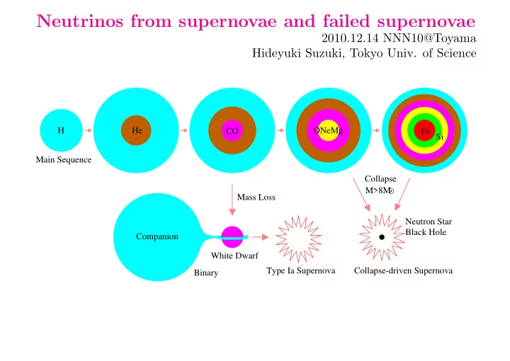
Neutrinos from supernovae and failed supernovae

2010.12.14 NNN10@Toyama Hideyuki Suzuki, Tokyo Univ. of Science

H M>8M Mass Loss Collapse He CO ONeMg Fe Si Neutron Star Black Hole Main Sequence Type Ia Supernova Collapse-driven Supernova White Dwarf Companion Binary

SLIDE 2

1 Collapse-Driven Supernova Explosion

SN Core (T ∼ 10MeV, ρ >

∼ 1014g/cm3)

τweak ≪ τdyn Neutrino Trapping

⇒ Neutrinos are also in thermal equilibrium and in chemical equilibrium nν ∼ nγ ∼ ne

mean free path length λν ≫ λγ, λe, λN

⇒ Neutrinos carry the energy and drive the evolution of the core ⇒ SN core can be seen by neutrinos (neutrinosphere) SN as a neutrino source

source of all species (νe,¯

νe,νµ,¯ νµ,ντ,¯ ντ)

T < O(100MeV) = mµ ⇒ ne− ≫ nµ, nτ: νx ≡ νµ, ¯

νµ, ντ, ¯ ντ

∫

Lνdt ∼ O(1053)erg ∼ 104Lν⊙τ⊙ ∼ 102Lγ⊙τ⊙ τ ∼ O(10)sec, d > O(1018)cm

Spectral difference: hierarchy of average energy(O(10)MeV)

σνe > σ¯

νe > σνx ⇒ ωνe<ω¯ νe<ωνx

Neutrinos pass through high density (matter and neutrinos) region(ρ = 0 ∼

1015g/cm3): High density MSW resonance, collective oscillation due to ν-ν interactions

SLIDE 3

Neutrinosphere ρ >10 g/cm

11 3 c Fe H He CO Si ONeMg

Fe core ρ

c=10 g/cm 9−10 3

νe

ν trapping (ρ > 1010 − 1012g/cm3) νe from e−A − → νeA′ and e−p − → νen main opacity source: coherent scattering νeA − → νeA cross section σ ∝ A2ω2

ν: λνA < λνN

(ν wave length ¯

hc Eν ∼ 20fm( Eν 10MeV)−1 ≫ nuclear size 1.2A

1 3 fm ∼ 5fm( A

56)

1 3 )

coherent scattering collapse

paque

trapping σ∼E^2 ν µ(ν) increase increase e capture suppress nuclei survive degenerate ν not so n−rich

Positive feedback (Sato 1975)

SLIDE 4

bounce >10 g/cm

14 3 c

ρ shock wave ν neutronization burst shock stall

e

ν(all) (collapse)~O(10−100)ms τ t(stall)=O(100ms) τ (neutronization burst)<O(10)ms Proto Neutron Star

Neutronization burst. Thompson et al., ApJ 592 (2003) 434 Fig.6 (failed explosion)

Shocked region A → np, e−p → nνe σ(e−A → νeA′) < σ(e−p → νen)

SLIDE 5

Prompt explosion (Hillebrandt, Nomoto and Wolff 1984). MMS = 9M⊙ Failed Prompt explosion (Hillebrandt 1987). MMS = 20M⊙

SLIDE 6

Wilson’s Delayed explosion model (Colgate 1989).

SLIDE 7

PNS cooling (PNS cooling)=O(10)s τ shock revival heating ν Hot Bubble νwind t(core exp.)=O(1)s Supernova Explosion t(SNE)=hours−day Neutron Star

SN1987A Crab nebula (remnant of SN1054)

SLIDE 8

Classical Simulations

Totani et al., 1998

early phase: hierarchy of average energy late phase: n-rich matter interacts ¯ νe and νx almost equally. degeneracy prohibits νe interactions, too.

neutrinos from protoneutron star cooling phase (Suzuki 2002)

SLIDE 9

Energetics

∆EG =

(

GM 2

core

RFe core − GM 2

core

RNS

) ∼ O(1053)erg

Ekin(obs.)∼O(1051)erg, Erad(obs.)∼O(1049)erg, EGW(sim.)∼O(1051)erg
rest O(1053)erg ∼ Eν
cf. Eν(SNIa) < 1049erg

νe’s from neutronization of all protons 26MFe core mFe Eνe ∼ 1.2 · 1052ergMFe core 1.4M⊙ Eνe 10MeV ∼ O(0.1) × Eν tot = ⇒ thermal ν ≫ neutronization νe = ⇒ νe, ¯ νe, νx: roughly equipartiton

SLIDE 10

Neutrino Transfer distibution function fνi(t, r, pν) (7 independent variables) ∂fν ∂tp + d r dtp ∂fν ∂ r + d pν dtp ∂fν ∂ pν = (∂fν ∂tp )

ν int.

Spherically symmetric case:

fνi(t, r, ων = pνc, µ = cos θ) (4 independent variables) ⇒ Fully general relativistic Boltzmann solver (Mezzacappa, Burrows, Janka, Sumiyoshi+Yamada >

∼ 2000)

Non-spherical case: 2D/3D ν transfer in progress

Neutrino Interactions (minimal standard: Bruenn’85) e−p ← → νen e+n ← → ¯ νep e−A − → νeA′ e+A − → ¯ νeA′ e−e+ ← → ν¯ ν plasmon ← → ν¯ ν NN − → NNν¯ ν νe¯ νe ← → νx¯ νx νN − → νN νA − → νA νe± − → νe± νν′ − → νν′

SLIDE 11

Equation of States (EOS) for high density matter (T = 0)

Lattimer-Swesty 1991: FORTRAN code

Liquid Drop model: Ks = 180, 220, 375MeV, Sv = 29.3MeV E/n ∼ −B + Ks(1 − n/ns)2/18 + Sv(1 − 2Ye)2 + · · ·

Shen’s EOS table (Shen et al., 1998)

RMF (n,p,σ, ρ, ω) with TM1 parameter set(gρ, · · ·) ⇐ Nuclear data includ- ing unstable nuclei ρB, nB, Ye, T, F, U, P, S, A, Z, M ∗, Xn, Xp, Xα, XA, µn, µp grids: wide range T = 0, 0.1 ∼ 100MeV ∆ log T = 0.1 Ye = 0, 0.01 ∼ 0.56 ∆ log Ye = 0.025 ρB = 105.1 ∼ 1015.4g/cm3 ∆ log ρB = 0.1 Extension with hyperons (Ishizuka, Ohnishi), quarks (Nakazato)

SLIDE 12

Modern Simulations Light ONeMg core + CO shell(1.38M⊙): weak explosion (O(1050)erg) (Progenitor: Nomoto 8-10M⊙) ν-heating + nuclear reaction ⇒ weak explosion

Fig. 1. Mass trajectories for the simulation with the W&H EoS as a

function of post-bounce time (tpb). Also plotted: shock position (thick solid line starting at time zero and rising to the upper right corner), gain radius (thin dashed line), and neutrinospheres (νe: thick solid; ¯ νe: thick dashed; νµ, ¯ νµ, ντ, ¯ ντ: thick dash-dotted). In addition, the composition interfaces are plotted with different bold, labelled lines: the inner boundaries of the O-Ne-Mg layer at ∼0.77 M⊙, of the C-O layer at ∼1.26 M⊙, and of the He layer at 1.3769 M⊙. The two dotted lines represent the mass shells where the mass spacing between the plotted trajectories changes. An equidistant spacing of 5×10−2M⊙ was chosen up to 1.3579M⊙, between that value and 1.3765M⊙ it was 1.3 × 10−3M⊙, and 8 × 10−5M⊙ outside.

Fig. 3. Velocity profiles as functions of radius for different post-

bounce times for the simulation with the W&H EoS. The insert shows the velocity profile vs. enclosed mass at the end of our simulation.

Kitaura et al., AAp 450(2006)345 (Mezzacappa’07: 11.2M⊙model explodes, too)

SLIDE 13

1 2 3 4 L [10

52 erg s

1]

10

2

10

1

10 0.05 0.1 0.15 0.2 8 10 12 <ε> [MeV] 2 4 6 8 5 10

νe νe νµ/τ L/10

Time after bounce [s]

Accretion Phase Cooling Phase

Neutrino luminosities and average energies at infinity for 8.8M⊙ progenitor.

L. H¨

udepohl et al., PRL104 (2010) 251101

SLIDE 14

Phase transition into quark matter

0.1 0.2 0.3 0.4 0.5 Time after bounce [s] 10 15 20 25 30 rms Energy [MeV] 1 Luminosity [10

53 erg/s]

0.255 0.26 0.265

Time after bounce [s]

1

Luminosity [10

53 erg/s]

FIG. 1: Neutrino luminosities and rms neutrino energies as

functions of time after bounce, sampled at 500 km radius in the comoving frame, for a 10 M⊙ progenitor star as modeled in [17]: νe in solid (blue), ¯ νe in dashed (red), and νµ/τ in dot-dashed (green). In contrast to the deleptonization burst just after bounce (t ∼ 5 ms) the second burst at t ∼ 257−261 ms is associated with the QCD phase transition. The inset shows the second burst blown up.

Dasgupta et al., PRD81 (2010) 103005

The second shock wave merges the first shock wave leading to explosion. ¯ νe > νe in the second burst (protonization)

SLIDE 15

Modern simulations with GR 1D Boltzmann ν-transfer canonical models: no explosion

0.1 0.2 0.3 0.4 0.5 10

1

10

2

10

3

Time After Bounce [s] Radius [km] Newton+O(v/c) Relativistic

NH 13M⊙, GR Boltzman, LS EOS+Si burning Liebend¨

rfer et al., Phys.Rev. D63 (2001) 103004

(astro-ph/0006418 v2) Fig.6

100 101 102 103 104 radius [km] 1.0 0.8 0.6 0.4 0.2 0.0 time [sec]

15M⊙, Shen EOS, Sumiyoshi et al., 2005.

Fig. 1.—Trajectories of selected mass shells vs. time from the start of the
simulation. The shells are equidistantly spaced in steps of 0.02 M,, and the

trajectories of the outer boundaries of the iron core (at 1.28 M,) and of the silicon shell (at 1.77 M,) are indicated by thick lines. The shock is formed at 211 ms. Its position is also marked by a thick line. The dashed curve shows the position of the gain radius.

WW 15M⊙, MFe = 1.28M⊙, NR Boltzmann (tangent-ray method), only νe,¯ νe, without e−e+ ↔ ν¯ ν, LS EOS, Rampp et al., ApJ 539 (2000) L33 Fig.1

Fig. 5.—Radial position (in km) of selected mass shells as a function of

time in our fiducial 11 M model.

NR 1D Boltzmann ν-transfer, Thompson et al., ApJ 592 (2003) 434 Fig.5

SLIDE 16

Comparison between Boltzmann solvers

Fig. 5.—(a) Shock position as a function of time for model N13. The shock in VERTEX (thin line) propagates initially faster and nicely converges after its maximum

expansion to the position of the shock in AGILE-BOLTZTRAN (thick line). (b) Neutrino luminosities and rms energies for model N13 are presented as functions of

time. The values are sampled at a radius of 500 km in the comoving frame. The solid lines belong to electron neutrinos and the dashed lines to electron antineutrinos. The

line width distinguishes between the results from AGILE-BOLTZTRAN and VERTEX in the same way as in (a). The luminosity peaks are nearly identical; the rms energies have the tendency to be larger in AGILE-BOLTZTRAN.

Liebend¨

rfer et al., ApJ620(2005)840 Fig.5

SLIDE 17

2 Failed supernovae

implicit GR hydrodynamics + Boltzmann ν transfer code

Sumiyoshi, Yamada, Suzuki, Chiba PRL97(2006) 091101

Fig. 1.—Radial trajectories of mass elements of the core of a 40 M star as a

function of time after bounce in the SH model. The location of the shock wave is shown by a thick dashed line.

Fig. 2.—Radial trajectories of mass elements of the core of a 40 M star as a

function of time after bounce in the LS model. The location of the shock wave is shown by a thick dashed line.

2x1053 1 luminosity [erg/s] 1.5 1.0 0.5 0.0 time after bounce [sec] 2x1053 1 luminosity [erg/s] 1.5 1.0 0.5 0.0 time after bounce [sec]

Lν increases due to matter accretion νx < νe, ¯ νe from ac- creted matter Burst duration time strongly depends on EOS!

Progenitor 40M⊙, left: Shen EOS, right: Lattimer-Swesty EOS 180

SLIDE 18

0.2 0.4 0.6 0.8 1 1.2 1.4 1 2 3 4 5 6 (a) Time After Bounce [s] Luminosity [1053 erg/s] 0.2 0.4 0.6 0.8 1 1.2 1.4 5 10 15 20 25 30 35 40 (b) Time After Bounce [s] rms Energy [MeV] e Neutrino e Antineutrino µ/τ Neutrinos

Figure 2. Luminosities and mean energies during the post bounce phase

f a core collapse simulation of a 40 M⊙ progenitor model from

Woosley and Weaver (1995). Comparing eos1 (thick lines) and eos2 (thin lines).

Fischer et al., 2008

SLIDE 19

Failed supernova neutrinos: expected observation by SK

Nakazato et al., PRD78 (2008) 083014

FIG. 5: Time-integrated spectra before the neutrino oscillation for models W40S (left) and W40L (right). Solid, dashed and

dot-dashed lines represent the spectra of νe, ¯ νe and νx, respectively.

FIG. 9 (color online).

Time-integrated spectra for the total event number of failed supernova neutrinos for the normal mass hierarchy with sin213 ¼ 108 (upper left), the normal mass hierarchy with sin213 ¼ 102 (upper right), the inverted mass hierarchy with sin213 ¼ 105 (lower left), and the inverted mass hierarchy with sin213 ¼ 102 (lower right). Results obtained without the Earth effects are shown. Solid, long-dashed, short-dashed, dot-dashed, and dotted lines represent models W40S, W40L, T50S, T50L, and H40L, respectively.

EOS (S,L), Progenitors (W40, T50, H40)

FIG. 8: Time-integrated total event number of failed supernova neutrinos for the normal mass hierarchy (left) and the inverted

mass hierarchy (right). Error bars represents the upper and lower limits owing to the different nadir angles. The upper and lower sets represent models W40S and W40L, respectively.

θ13 dependence for W40S vs. W40L

SLIDE 20

hyperon EOS vs. soft nucleon EOS

10-5 10-4 10-3 10-2 10-1 100 20x105 10 radius [km] Λ Ξ− n p α Σ− Ξ0 Σ0 Σ+ 20 10-5 10-4 10-3 10-2 10-1 100 20x105 10 radius [km] Λ Ξ− n p α Σ− Ξ0 Σ0 Σ+ 20

Fig. 2.— Mass fractions of hyperons in model IS are shown as a function of radius at tpb=500

(left) and 680 ms (right).

50 40 30 20 10 < Eν > [MeV] 2x1053 1 Lν [erg/s] 1.5 1.0 0.5 0.0 time after bounce [sec]

Fig. 3.— Average energies and luminosities of νe (solid), ¯

νe (dashed) and νµ/τ (dash-dotted) for model IS are shown as a function of time after bounce. The results for model SH and LS are shown by thin lines with the same notation.

Sumiyoshi et al., Astrophys. J. 690 (2009) L43-L46

increase of degree of freedom → Soft EOS Hyperon EOS vs. Lattimer-Swesty EOSs (LS180/220)(Nakazato et al., 2010) might be distinguishable by the time pro- file Good probe to properties of high density matter

SLIDE 21

3 Non-spherial explosion

SN1987A observations

polarization
material mixing (large vFe > 3000km/sec(Fe II IR line), early detection of

X-ray, 847keV/1238keV 60Co line), slow H velocity (∼ 800km/sec)

asymmetric image

⇒ fluid instability, rotation, magnet field: multi-dimensional simulation

HST image of SN1987A on 1994.2 and 2003.11.28

SLIDE 22

Nomoto et al., astro-ph/0308136

SLIDE 23

2D/3D Hydrodynamics + simplified ν-transfer + full/approximated GR At present, evolution of fν(t, r, pν) cannot be calculated. SASI: Standing Accretion Shock Instability Blondin et al., 2003 Instability modes with ℓ = 1, 2 grow between stalled shock wave and pro- toneutron star (amplifying advective-accoustic cycle) It helps neutrino heating (longer advection time)

?

⇒ successful explosion Accoustic Explosion? Burrows et al., 2006 accretion → excitation of g-mode in PNS → sound wave → dissipation behind the shock front

?

→ robust explosion rotation/magnetic field? Angular momentum of core might be small (Heger et al., 2005) jet-like explosion by non-spherical neutrino heating? suppresion of instability due to rotation? practically strong magnetic field

?

→ Magnetar (B = 1015G) Many groups are at work. Garching, LANL, ORNL, Basel, Prince- ton/Caltech, NAOJ/Waseda, Kyoto ...

SLIDE 24

Janka et al.., 2006, non-rotating 11.2M⊙ 2D simulation ⇒ weak explosion due to SASI+ν-heating Simulation for π

4 ≤ θ ≤ 3π 4 does not explode, 0 ≤ θ ≤ π: explodes

instability modes with l = 1, 2(SASI) evolve → kick velocity?

entropy profiles: Janka et al., astro-ph/0612072

τadv ր> τheat, wider heating region: SASI helps ν-heating

SLIDE 25

Marek et al., Astron. Astrophys. 496 (2009) 475

60 120 180

4•109
2•109

2•109 180 120 60 5 10 15 20

s[kB/baryon] vr [cm/s] r [km]

60 120 180

4•109
2•109

2•109 180 120 60 5 10 15 20

s[kB/baryon] vr [cm/s] r [km]

60 120 180

4•109
2•109

2•109 180 120 60 5 10 15 20

s[kB/baryon] vr [cm/s] r [km]

60 120 180

4•109
2•109

2•109 4•109 180 120 60 5 10 15 20 25

s[kB/baryon] vr [cm/s] r [km]

Fig. 3. Four representative snapshots from the 2D simulation with the L&S EoS at post-bounce times of 247 ms (top left), 255 ms (top right),

322 ms (bottom left), and 375 ms (bottom right). The lefthand panel of each figure shows color-coded the entropy distribution, the righthand panel the radial velocity component with white and whitish hues denoting matter at or near rest; black arrows in the righthand panel indicate the direction of the velocity field in the post-shock region (arrows were plotted only in regions where the absolute values of the velocities were less than 2 × 109 cm s−1). The vertical axis is the symmetry axis of the 2D simulation. The plots visualize the accretion funnels and expansion flows in the SASI layer, but the chosen color maps are unable to resolve the convective shell inside the nascent neutron star.

100 200 300 400 50 100 150 200 250

Rs,max [km], Rns [km] tpb [ms] L&S-EoS H&W-EoS

250 -150

50 50 150 250

200
100

100 200

Rs [km] Rs [km] Rs [km] L&S-EoS H&W-EoS

248 ms 270 ms 300 ms 319 ms 380 ms

Fig. 4. Left: maximum shock radii (solid lines) and proto-neutron star radii (dashed lines) as functions of post-bounce time for the 2D simulations

with different nuclear equations of state. The neutron star radii are determined as the locations where the rest-mass density is equal to 1011 g cm−3. Right: shock contours at the different post-bounce times listed in the figure. The vertical axis of the plot is the symmetry axis of the simulation.

SLIDE 26