
SLIDE 1
Universality of step bunching behavior in systems with non-conserved dynamics
Joachim Krug Institute for Theoretical Physics, University of Cologne
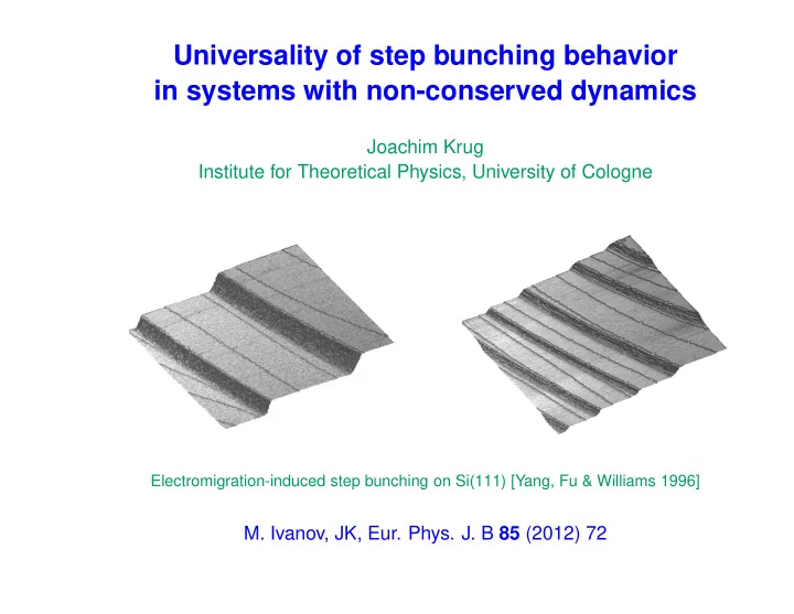
Electromigration-induced step bunching on Si(111) [Yang, Fu & Williams 1996]
- M. Ivanov, JK, Eur. Phys. J. B 85 (2012) 72