
SLIDE 1
Unit 2: Probability and distributions
- 3. Normal and binomial distributions
Sta 101 - Spring 2019
Duke University, Department of Statistical Science
- Dr. Abrahamsen
Slides posted at https://stat.duke.edu/courses/Spring19/sta101.002
Announcements ▶ RA 3 on Tuesday ▶ PS 2 due Friday, PA 2 due Sunday
1
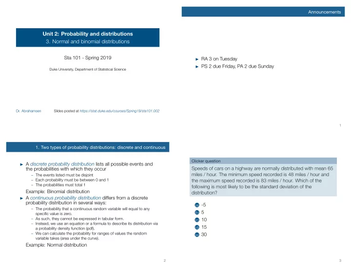
- 1. Two types of probability distributions: discrete and continuous