
SLIDE 1
ST 516 Experimental Statistics for Engineers II
Checking Assumptions
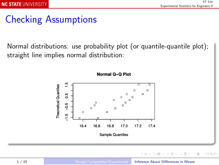
Normal distributions: use probability plot (or quantile-quantile plot); straight line implies normal distribution:
16.4 16.6 16.8 17.0 17.2 17.4 −1.5 −0.5 0.5 1.5
Normal Q−Q Plot
Sample Quantiles Theoretical Quantiles
- 16.4
16.6 16.8 17.0 17.2 17.4 −1.5 −0.5 0.5 1.5
Normal Q−Q Plot
Sample Quantiles Theoretical Quantiles 1 / 15 Simple Comparative Experiments Inference About Differences in Means