Ultrafast spectroscopy Detector Stuff Generally you have some - - PowerPoint PPT Presentation

Detector

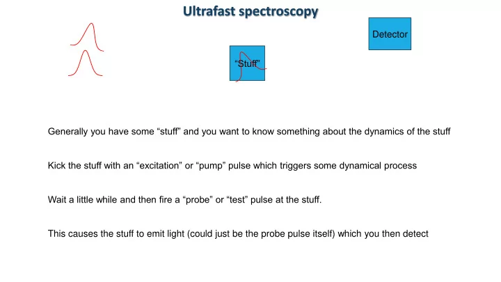
Ultrafast spectroscopy

Generally you have some “stuff” and you want to know something about the dynamics of the stuff “Stuff” Kick the stuff with an “excitation” or “pump” pulse which triggers some dynamical process Wait a little while and then fire a “probe” or “test” pulse at the stuff. This causes the stuff to emit light (could just be the probe pulse itself) which you then detect

Nonlinear spectroscopy

Linear: absorption, reflection, fluorescence/luminescence Nonlinear: two or more laser beams interact with each other in the sample Interaction only occurs if the response of the sample to light is nonlinear (otherwise superposition principle holds) Why use nonlinear spectroscopic techniques? Because they produce more information, for example:

• Homogeneous linewidth in an inhomogeneously broadened sample
• Dynamics such as relaxation or diffusion
• Coupling or lack of coupling between resonances
• Access to multiply excited states or forbidden transitions

They generally require relatively high intensities in at least on beam, thus only possible using lasers Generally can be implemented in either time or frequency domains. Most ultrafast spectroscopy techniques are a form of “nonlinear spectroscopy”

Time versus frequency

Time Frequency Vary delay between pulses in two beams Vary frequency difference between two CW beams Easy: short delays ( < 1 ns) Easy: small detunings (< 1 GHz) Hard: large delays (> 5 ns) Hard: Large detunings (> 3 GHz) Furthermore: consider what happens when there are two timescales:

Signal Delay

Exponential Decays with fast timescale slow timescale

Signal Detuning

Lorentzians with widths inversely proportional to Slow timescale Fast timescale

Tends to get lost in the noise More sensitive to fastest process More sensitive to slowest process Conclusion Better for fast processes Better for slow processes

Incident pulses

“Hey …this is ultrafast, isn’t the shortest possible pulse always the best?” ….is it?.....

• No. Generally not.

Generally the best is to use the longest pulse you can get away with: it needs to be short enough to resolve the fast dynamics, but no shorter. Why? 1) It will “drive” the system better. Spectral domain: better overlap between pulse spectrum and absorption spectrum Time domain: coherently build up excitation up to dephasing time (1/linewidth) 2) Give some ability to spectrally select the resonance of interest Most of the time there are other states/transitions at different energies, exciting them can lead to confusion. What is the optimum duration for the incident pulses?

Detection

Detection can generally be categorized as (in increasing order of difficulty): 1) Time & spectrally integrated Detect energy of emitted signal pulses Average over many pulses 2) Spectrally resolved Typically just a grating spectrometer 3) Temporally resolved Usually done with cross correlation, cross-FROG 4) Full characterization of electric field Spectral interferometry with phase locked reference pulse Spectrally or Temporally resolved detection provides more information, and are typically related (FT) Question: Do they provide useful additional information? Answer: It depends….

Incoherent versus coherent spectroscopy

Incoherent: only sensitive to “population” relaxation  rate equations sufficient Examples: Time resolved fluorescence/luminescence Transient absorption Spectrally resolved transient absorption Transient grating Coherent: also sensitive to phase relaxation  Optical Bloch Equations needed Example: Transient Four-wave Mixing (a.k.a. Photon Echoes) Two-dimensional Fourier Transform spectroscopy

Time resolved fluorescence/luminescence

Uses a single pulse Is linear Excite high lying state/band with short pulse Time resolve spontaneously emitted fluorescence from lower state Energy difference of absorbed and emitted photon needed to distinguish scattered pump photons from spontaneously emitted photons Rise time of fluorescence gives g21 Decay gives g10 Challenge: detection with sufficient time resolution 1) Time-correlated photon counting 2) Streak camera 3) Up-conversion/cross-correlation Fluor. Pump

1 2

g21 g10 Only technique that

Time-correlated single photon counting I

1) Excite sample with short pulses 2) Collect less than 1 photon of fluorescence per pulse 3) Record time of arrival (relative to excitation pulse) of fluorescence photons 4) Repeat and build up histogram of arrival times (#photons per time bin) Spectr.

Det. Det. Time-to- amplitude converter Start Stop Excitation pulses

Challenges: Temporal dispersion in single photon detector

PMT Microchannel plate

Temporal dispersion in spectrometer Amplitude fluctuations

Use constant fraction discrimator

Time-correlated single photon counting II

Measurement is convolution of actual decay function with system response function Spectr.

Det. Det. Time-to- amplitude converter Start Stop Excitation pulses

System Response Function Luminescence

     dt

t G t S H



   

H() – measured histogram S() – system response function G() – Fluorescence decay function Generally 1) assume functional form for G() (multi-exponential) 2) fit H() 3) using a measured S() (use scatterer – instantaneous) Best achieved time resolution with MCP ~ 30 ps

Streak camera

Convert light to electrons Use electric field ramp to streak electrons across phosphor screen Synchronize ramp to excitation pulse Converts time to space Similar technology to oscilloscope Often use 2D screen, wavelength in other axis Best time resolution: 200 fs Typical resolution: few ps Typical results Note rise time for horizontal polarized, time for molecules to reorient

Upconversion

Cross-correlation between fluorescence and a reference pulse Overlap in second harmonic crystal, detect sum frequency light as function of reference pulse delay Excellent time resolution limited only by: Pulse duration Geometric considerations in overlap Limitation: Limited “acceptance angle” of phase matching

 Wang, Shah, Damen and Pfeiffer, Phys. Rev. Lett. 74, 3065 (1995)

Transient Absorption

Standard explanation: Absorption of a two level system is proportional to n0 – n1 If the pump pulse excites population into upper state, n0 decreases, n1 increases, so absorption decreases. Signal as a function of delay gives relaxation rate of upper state back to lower state I(t) I(t–) Signal is DT =(transmission of probe with pump) – (transmission of probe without pump) This is implemented using an optical chopper and lockin detection Typically actual measurement is Lockin

DET lockin l

I S e T T    D

D 

1



Directly related to change in absorption coefficient, easy to measure Pump

1

Transient Absorption

Generally keep probe weaker than pump

(not needed in “c(3)” regime)

Signal should be Proportional to pump intensity Proportional to probe intensity I(t) I(t–) Lockin

Spectrally resolved Transient Absorption

Similar to transient absorption, but take spectrum of transmitted probe at each delay Again take difference between spectrum with pump and without pump Particularly effective for tracking excitation in bands I(t) I(t–) Shutter For resonances: Sensitive to, and can differentiate between, more mechanisms than just “saturation” (also known as bleaching) Bleaching: change in oscillator strength Broadening: change with linewidth Spectral shift: change in center frequency

Spectrally resolved transient absorption lineshapes

Each mechanism gives different lineshape Note: Area is zero for broadening or spectral shift  no signal for spectrally integrated

w0 G

f SRTA Signal Frequency    

4 2 1 ~

2 2

G   G w w  w f P

1.37 1.38 1.39 1.40

• 0.2

0.0 0.2 0.4 0.6 0.8 1.0

Fit

Normalized Transient Abs. Signal Photon Energy (eV)

Transient Absorption: Excited state absorption

Additional signal due to excited state absorption Induced absorption because transitions to higher lying states becomes allowed

Pump 1 2 Probe

Transient grating

Interfere two beams: form grating in excited state population. Decays due to: Relaxation from upper to lower state And, due to diffusion with decay constant

2 2

4   G D

D



Where D is diffusion rate,  is inverse grating spacing

Raman Scattering

The frequency of light can shift on scattering from a medium Leaves an “excitation” behind in the medium to conserve energy Molecular vibration Phonon Magnon etc… First observed in 1928 by C.V. Raman (on February 28th, to be exact) Used sunlight (no lasers in 1928) Tends to be a very weak effect So lasers helped a lot….

Incident “pump” photon Raman photon

Energy of “excitation”

Typical Spontaneous Raman Scattering Experiment

Relatively high power laser Really, really good monochrometer Raman shifts are typically relatively small Raman effect is weak Difficult to separate Raman signal from incident laser light Typically requires photon counting level detection Raman spectra give Energy of “excitation” Width (= lifetime) of excitation Laser

Raman vs. Fluorescence

leaves atom in an excited state …or…heats material (relaxation in upper state) How do you distinguish between Raman and Fluorescence? 1) Raman does not require a “real” upper state 2) Raman is a coherent and “instantaneous” process 3) Raman intensity scales as w4 4) Raman obeys “strict” selection rules in polarization and momentum 5) Raman transitions are not optically allowed “Resonant” Raman blurs these distinctions Fluorescence Raman Fluorescence can also produce light of a different color

Stimulated Raman

In “Stimulated” Raman, the laser field(s) drives both transitions This creates coherence among the excitations The coherence is then probed with another laser field (could actually be same laser) Observed as a higher order scattering process “Anti-Stokes Raman Scattering” Or by change in properties of other laser field, usually phase Ultrafast pulses: can have enough bandwidth that both photons come from a single pulse This means that the pulse duration is shorter than one oscillation of the “excitation” Impulsive regime: pulse is more than a factor of 2 shorter In molecules this means that multiple vibrational levels are excited and a “wavepacket” is created

Molecular vibrations: driving pulse

Short pulse starts the molecule vibrating Oscillations in the THz frequency range Semi-classically: Impulsive kick Occurs because pulse mixes in excited state with shifted potential minimum Quantum Mechanically: Raman Transition between vibrational quantum states

Internuclear distance

Ground state Potential Energy Excited state Potential Energy

Internuclear distance

Ground state Potential Energy Excited state Potential Energy

Detection with a probe pulse

Classical picture: Polarizability of bond depends on intranuclear separation Polarizability is responsible for index of refraction  vibration corresponds to oscillating bond length which results in oscillating index of refraction Oscillating index of refraction phase modulates pulse Dibromomethane

Ruhman, Joly, Williams and Nelson, Rev. Phys. Appl. 22, 1717 (1987)

Pulse is shorter that oscillation time  pulse sees phase ramp, which is frequency shift Narrow filter converts oscillating frequency into amplitude Example at right shows opposite sides of probe spectrum Quantum picture: Raman transitions Alternates between Stokes and anti-Stokes depending on phase of Raman coherence

Optical Phonons

Similar to molecular vibrations Effectively molecules on lattice Optical phonons basically don’t propagate Short pulse excites phonon Effectively standing wave Called “Coherent Phonons” Often use “spectrally resolved” detection

Example of coherent phonons

Phonons in LaAlO3

Liu, et al., Phys. Rev. Lett. 75, 334 (1995).

Transmission signal due to “boundary” effects i.e., change in reflectivity Shows temperature dependence of Phonon frequency (earlier slide) Phonon decay rate Both compare well with Raman scattering

Magneto-Optical Faraday Effect

Observed by Faraday in 1845 The polarization of light propagating parallel to a magnetic field in a material rotates magnitude of rotation proportional to field rotation direction depends of field direction, not propagation direction Simple classical description for transparent materials: Decompose linearly polarized light into left and right handed circular components Circular component makes electron execute circular motion Magnetic field either causes the orbit radius to increase or decrease depending on direction relative to field

Increase in radius means stronger interaction  larger index of refraction Decrease in radius means weaker interaction  smaller index of refraction

Difference in refraction corresponds to a relative phase shift, resulting in rotation of linear polarization

Magneto-optical Kerr Effect

Observed by Rev. John Kerr in 1877 Reflected linearly polarized light off of polished electromagnet pole Observed that the polarization rotated Amount of rotation proportional to field Rotation direction switched with a switch in field direction Basically, the magneto-optic Kerr effect is the reflected version of the magneto-optic Faraday effect In both Faraday and Kerr effects there is both a Rotation of the polarization direction and Change in ellipticity These have opposite origins in the two cases…

Transient Faraday/Kerr Effect

In ultrafast, the photo- Faraday or Kerr effect is of interest The broken symmetry between right and left handed components is induced by light Due to a pump, which is generally circularly polarized Simplest case: resonances that differ in angular momentum, circularly polarized pump saturates one of them Furthermore, if that is done with a short pulse, we can watch relaxation Example: spin flips of electrons A magnetic field is generally not required, although one may be used

Resonant Faraday and Kerr effect

Consider the absorption and index of refraction for a simple resonance For no magnetic field both helicities see same resonance Static magnetic field Zeeman effect will shift one up in frequency the other down This creates a difference in index (and absorption) for light

• f a single frequency

Taking the difference between right and left gives the Faraday and Kerr effects Faraday rotation: Difference between index Faraday ellipticity: Difference between absorption Kerr ellipticity: difference between index Kerr rotation: difference between absorption

• 4
• 2

2 4

(b) Rotation (a.u.) Detuning (ww)/g Kerr Faraday (a) Faraday (a.u.) ellipticity rotation

• 1.0
• 0.5

0.0 0.5 1.0 0.0 0.2 0.4 0.6 0.8 1.0

Detuning Absorption Coefficient Index of Refraction

• 1.0
• 0.5

0.0 0.5 1.0 0.0 0.2 0.4 0.6 0.8 1.0

Detuning Absorption Coefficient Index of Refraction Right handed Left handed

Transient Faraday/Kerr

Circularly polarized pump beam creates excitation of one handedness Saturates that resonance

• r, creates effective magnetic field (aligned spins)
• r, there is spin-dependent scattering

Measure signal as a function of delay between pump pulse and probe pulse Data at right shows signal when applied magnetic field is perpendicular to propagation direction electrons precess around field precession frequency yields g-factor

Faraday rotation/ellipticity versus transient absorption

There is clearly a close connection between Faraday/Kerr rotation or ellipticity and transient absorption Faraday/Kerr rotation is sensitive to changes in index of refraction Other polarization acts as “local oscillator” Advantages over transient absorption: Far off resonance, index changes are larger than absorption changes Utilizes “balanced” detection so amplitude fluctuations on input laser are cancelled Quite small rotations can be measured

1.535 1.540 1.545

• 20
• 10

10

Faraday (mrad)

Faraday rotation/ellipticity as a Raman process

It is possible to view Faraday and Kerr experiments on spin systems as Raman processes Lower two levels are spin up versus spin down Pump photon imparts angular momentum and energy necessary to make transition from spin down to spin up

Cool example of Faraday rotation in “spintronics”

Drag spin polarized electrons using a transverse electric field

Kikkawa and Awschalom, Nature 397, 139 (1999)