[PPT] - Two-fluid 20-moment simulation of fast magnetic reconnection E. Alec PowerPoint Presentation

SLIDE 1

Two-fluid 20-moment simulation of fast magnetic reconnection

E. Alec Johnson

Department of Mathematics KU Leuven These slides were presented in my behalf at CSE13 in Boston Massachusetts on February 25, 2013 Abstract. The 20-moment two-fluid-Maxwell model resolves diagonal pressure tensor components near the X-point when compared with Vlasov simulations of fast magnetic reconnection, in contrast to the 10- moment model. This occurs because, unlike the hyperbolic 10-moment model, the 20-moment model admits heat flux, which is a modeling re- quirement to admit steady-state 2D symmetric (driven) magnetic reconnection.

Johnson (KU-Leuven) 20-moment two-fluid reconnection

Feb. 25, 2013

1 / 56

SLIDE 2

Outline

1 Hyperbolic plasma models 2 Magnetic reconnection: Vlasov vs. fluid simulations Johnson (KU-Leuven) 20-moment two-fluid reconnection

Feb. 25, 2013

2 / 56

SLIDE 3

Standard of truth: 2-species kinetic-Maxwell (classical)

Maxwell’s equations: ∂tB + ∇ × E = 0, ∂tE − c2∇ × B = −J/ǫ, ∇ · B = 0, ∇ · E = σ/ǫ. Charge moments: σ :=

s qs ms

fs dv,

J :=

s qs ms

vfs dv.

Kinetic equations: ∂tfi +v · ∇xfi +ai · ∇vfi = Ci ∂tfe+v · ∇xfe+ae · ∇vfe= Ce Lorentz acceleration: ai = qi

mi (E + v × B) ,

ae = qe

me (E + v × B) .

BGK collision operator Cs = fθ − fs τs , where fθ = ρ (2πθ)3/2 exp −|c|2 2θ

,

θ := |c|2/2.

Johnson (KU-Leuven) 20-moment two-fluid reconnection

Feb. 25, 2013

3 / 56

SLIDE 4

Fluid approximation requires a numerical collision operator

Fluid models are kinetic equation solvers. Characteristic speeds correspond to discrete velocities. Fluid models evolve moments. Moments define a representation Fs selected from a finite-dimensional space F. convergence Fs → fs requires an infinite number of moments. F is a good representation space when C is large but bad when C is small. How can we justify fluid models when physically Cs = 0? by a multiscale framework: fluid models are a coarse-scale model used to accelerate convergence of the lowest moments

f the kinetic equation.

Cs can be physically defined to incorporate all microscale effects not resolved by the coarse-scale model. in code, Cs = 0 is a numerical mechanism to regularize fs. collision period τs selects the largest time scale for resolution of velocity-space detail. How to choose Cs? use a simple choice based on what you want to resolve. BGK damps all components and moments representing perturbation from Maxwellian at the same rate τ −1

s

. Damping individual moments at tunable rates allows smooth transition to a model with more moments. Faster damping for higher moments corresponds to faster damping for finer-scale components of fs.

Johnson (KU-Leuven) 20-moment two-fluid reconnection

Feb. 25, 2013

4 / 56

SLIDE 5

Conserved Moment Evolution

Convention: Products and powers of vectors are defined by tensor products. Conserved moments are moments of monomials in v. Let χ = χ(v). Take the χth moment of the kinetic equation:

v

χ

∂tf + ∇x·(vf) + ∇v·(af) = C
Integrate by parts to get

∂t

vχf + ∇·
vvχf =
vfa · ∇vχ +
vχC

(1) Choose χ = vn. Define

Fn :=
v

vnf,

Cn :=
v

vnC. Since a = q

m (E + v × B),

a · ∇v(vn) ∨ = q

m n

Evn−1 + vn × B
.

Substituting into equation (1) gives: General conserved moment evolution ∂t Fn + ∇· Fn+1 ∨ = q

m n

E

Fn−1 + Fn × B

+

Cn This is a hierarchy of moment evolution equations: ∂t F0 + ∇· F1 = C0, ∂t F1 + ∇· F2 = q

m (E

F0 + F1 × B)+ C1, ∂t F2 + ∇· F3 ∨ = q

m 2

E

F1 + F2 × B

+

C2, ∂t F3 + ∇· F4 ∨ = q

m 3

E

F2 + F3 × B

+

C3, ∂t F4 + ∇· F5 ∨ = q

m 4

E

F3 + F4 × B

+

C4. Tensor notation: AB = A ⊗ B = tensor product, Sym A = symmetrization of tensor A, A ⊻ B = Sym(A ⊗ B), and A ∨ = B ⇐ ⇒ Sym A = Sym B.

Johnson (KU-Leuven) 20-moment two-fluid reconnection

Feb. 25, 2013

5 / 56

SLIDE 6

Primitive moments

Fluid closures should be Galilean invariant. The kinetic equation is Galilean-invariant, so we require fluid closures to be Galilean-invariant. Primitive moments are Galilean-invariant Definitions: ρ =

v

f χ :=

v χ

ρ u := v c := v − u Fn :=

v

cnf Specifying closure in terms of primitive moments Fn ensures that closures are Galilean-invariant.

Johnson (KU-Leuven) 20-moment two-fluid reconnection

Feb. 25, 2013

6 / 56

SLIDE 7

Mapping from conserved to primitive variables

To express primitive moments in terms of conserved moments we observe that cn ∨ =(v − u)n ∨ =

n

j=0

(−1)jn j

ujvn−j.

Multiplying by C and integrating over velocity, C0= C0, C1= C1 − u C0, C2 = C2−2u C1 + u2 C0, C3 ∨ = C3 − 3u C2+3u2 C1 − u3 C0, C4 ∨ = C4 − 4u C3 + 6u2 C2−4u3 C1 + u4 C0, where in the absence of production C0 = 0 and in the further absence of interspecies friction C1 = 0. Multiplying by f and integrating over velocity, F0 = ρ, F1 = 0, F2 = F2 − ρu2, F3 ∨ = F3 − 3u F2 + 2ρu3, F4 ∨ = F4 − 4u F3 + 6u2 F2 − 3ρu4, F5 ∨ = F5 − 5u F4 + 10u2 F3 − 10u3 F2 + 4ρu5, where we have used that F1 = ρu. In practice, when computing with conserved variables, we compute the primitive variables that we need for the closing moment and then use one of the relations

F3 ∨

= F3 + 3u F2 − 2ρu3,

F4 ∨

= F4 + 4u F3 − 6u2 F2 + 3ρu4,

F5 ∨

= F5 + 5u F4 − 10u2 F3 + 10u3 F2 − 4ρu5 to solve for the closing conserved moment.

Johnson (KU-Leuven) 20-moment two-fluid reconnection

Feb. 25, 2013

7 / 56

SLIDE 8

Mapping from primitive to conserved variables

To express conserved moments in terms of primitive moments we observe that vn ∨ =(u + c)n ∨ =

n

j=0

n j

ujcn−j.

Multiplying by C and integrating over velocity,

C0= C0,
C1= C1 + uC0,
C2 = C2+2uC1 + u2C0,
C3 ∨

= C3 + 3uC2+3u2C1 + u3C0,

C4 ∨

= C4 + 4uC3 + 6u2C2+4u3C1 + u4C0, where in the absence of production C0 = 0 and in the absence of interspecies friction C1 = 0. Multiplying by f and integrating over velocity,

F0 = ρ,
F1 = ρu,
F2 = F2 + ρu2,
F3 ∨

= F3 + 3uF2 + ρu3,

F4 ∨

= F4 + 4uF3 + 6u2F2 + ρu4,

F5 ∨

= F5 + 5uF4 + 10u2F3 + 10u3F2 + ρu5, where we have used that F1 = 0.

Johnson (KU-Leuven) 20-moment two-fluid reconnection

Feb. 25, 2013

8 / 56

SLIDE 9

Collisional closures

Conventional names for primitive moments: P := F2, Q := F3, R := F4, S := F5, δtP := C2, δtQ := C3, δtR := C4. Collisional moments for BGK collision operator: δtP = − P◦ τ , δtQ = − Q τ3 , δtR

∨

= 3PP/ρ − R τ4 , where P◦ := P − pI is deviatoric pressure and for BGK τ = τ3 = τ4. Model coarsening: dial τ4 ց 0 to smoothly transition from 35-moment to 20-moment model. dial τ3 ց 0 to smoothly transition from 20-moment to 10-moment model. dial τ ց 0 to smoothly transition to the 5-moment model. and where when computing Cn =

c cn(fθ − f)
τ

we have used that

c

fθ = ρ,

c

cfθ = 0,

c

ccfθ = P

c

cccfθ = 0, and

c

ccccfθ

∨

= 3PP/ρ.

Johnson (KU-Leuven) 20-moment two-fluid reconnection

Feb. 25, 2013

9 / 56

SLIDE 10

20-moment flux closure

20-moment Maxwellian-based closure [Grad49] R

∨

= 3(PP − P◦P◦)/ρ. 20-moment Gaussian-based closure [GrothGRB03] R

∨

= 3PP/ρ . Comparison of closures: The Maxwellian-based closure assumes that the velocity distribution is a Maxwellian times a polynomial. The Gaussian-based closure assumes that the velocity distribution is a Gaussian times a polynomial. Gaussian-based closure is a consistent generalization of the 10-moment model. Gaussian-based closure is hyperbolic if heat flux is small enough. Maxwellian-based closure is hyperbolic if heat flux and deviatoric stress are small enough. BGK would relax R to the Gaussian-based closure for R.

Assumed distributions Entropy-maximizing closure: f(c) = exp(a · m), where m = (1, cc, ccc) is the tuple of evolved moments and a is a tuple of coefficients. Maxwellian-based closure f = WM (1 + c′ · m), where WM := exp(c0 · m0), m0 = (1, |c|2), and c′ · m is a polynomial orthogonal to 1 and |c|2 in the weight WM . Gaussian-based closure f = WG(1 + c′ · m), where WG := exp(c0 · m0), m0 = (1, cc), and c′ · m is a polynomial orthogonal to 1 and cc in the weight WG.

Johnson (KU-Leuven) 20-moment two-fluid reconnection

Feb. 25, 2013

10 / 56

SLIDE 11

35-moment flux closure (aside)

35-moment Gaussian-based closure [GrothGRB94] S

∨

= 10ΘQ , where Θ := P/ρ. Remarks: Thoroughly studied in [GrothGRB94] and [Brown96]. Large hyperbolicity region containing a Gaussian. Simple eigenstructure.

Assumed distributions Entropy-maximizing closure: f(c) = exp(a · m), where m = (1, cc, ccc, cccc) is the tuple of evolved moments and a is a tuple of coefficients. Maxwellian-based closure f = WM (1 + c′ · m), where WM := exp(c0 · m0), m0 = (1, |c|2), and c′ · m is a polynomial orthogonal to 1 and |c|2 in the weight WM . Gaussian-based closure f = WG(1 + c′ · m), where WG := exp(c0 · m0), m0 = (1, cc), and c′ · m is a polynomial orthogonal to 1 and cc in the weight WG.

Johnson (KU-Leuven) 20-moment two-fluid reconnection

Feb. 25, 2013

11 / 56

SLIDE 12

Primitive moment evolution equations (aside)

Take primitive moments of the kinetic equation. Relations for primitive moments: c(t, x, v) := v − u(t, x)

v

=

c

χ(t, x, v) = χ(c) = cn ∇vχ = ∇cχ dv

t

:= ∂t + v · ∇x ρα :=

vα

Dt (α) := ∂t α + ∇x·(vα) + ∇v·(aα) Dt := ∂t + v · ∇x + a · ∇v = Dt Dt (αβ) = (Dt α)β + αDt β Multiply the kinetic equation Dt f = C by χ to get Dt (χf) = fDt χ + χC. (2) But observe that for χ(c): Dt = dv

t + a · ∇v·,

dv

t χ = (dv t c) · ∇cχ

= −(dv

t u) · ∇cχ,

dv

t = du t + c · ∇x;

putting it together, Dt χ = a − du

t u − c · ∇xu

·∇cχ (3) But solving momentum evolution ρdu

t u + ∇·F2 = ρa + C1

for du

t u, substituting in (3), and defining

a′ := a − a = q

m c × B

gives Dt χ = a′ − c · ∇xu · ∇cχ + ∇·F2 − C1 ρ · ∇cχ. (4)

Substituting (4) into the kinetic equation (2) and integrating over velocity space yields: ∂t(ρχ) + ∇·(ρuχ) + ∇·(ρcχ) = (∇·F2 − C1) · ∇cχ + ρ a′ − c · ∇u

· ∇cχ
+
vχC.

(5) Now impose that χ(c) = cn. For a generic α, α · ∇c

cn

= n Sym

αcn−1

. So ρ

(a′ − c · ∇u) · ∇ccn

= nρ Sym

(a′ − c · ∇u)cn−1

= n Sym q

m Fn × B − Fn · ∇u

(6)

Substituting identity (6) into equation (5) gives an evolution equation for primitive moments: ρdtFn + n Sym

Fn−1(C1 − ∇·F2) + Fn · ∇u
+ ∇·Fn+1 = n Sym

q

m Fn × B

+ Cn,

(7) where Fn := cn = Fn/ρ. and dt := ∂t + u · ∇.

Johnson (KU-Leuven) 20-moment two-fluid reconnection

Feb. 25, 2013

12 / 56

SLIDE 13

Primitive quasilinear form (aside)

Equation (7) can also be written: ρdtFn − nFn−1∇·F2 + nFn · ∇u + ∇·Fn+1 ∨ = n q

m Fn × B − nFn−1C1 + Cn ,

which is an evolution equation for the generalized temperature Fn. The 35-moment system in quasilinear form is thus dtρ + ρ∇·u = C0 = 0, ρdtu + ∇·F2 =

q m ρ(E + u × B) + C1,

ρdtF2 + 2F2 · ∇u + ∇·F3 ∨ = 2 q

m F2 × B + C2,

ρdtF3 − 3F2∇·F2 + 3F3 · ∇u + ∇·F4 ∨ = 3 q

m F3 × B − 3F2C1 + C3,

ρdtF4 − 4F3∇·F2 + 4F4 · ∇u + ∇·F5 ∨ = 4 q

m F4 × B − 4F3C1 + C4,

which generalizes equations (4.15) through (4.19) in [GrothGRB03] and agrees if C0 = 0 (as implicitly assumed

n the previous slide).

Johnson (KU-Leuven) 20-moment two-fluid reconnection

Feb. 25, 2013

13 / 56

SLIDE 14

Outline

1 Hyperbolic plasma models 2 Magnetic reconnection: Vlasov vs. fluid simulations Johnson (KU-Leuven) 20-moment two-fluid reconnection

Feb. 25, 2013

14 / 56

SLIDE 15

Magnetic Reconnection

Magnetic field lines are convected with plasma except near reconnection point. Adjacent oppositely directed magnetic field lines field lines come together and cancel and reconnect. Oppositely directed jets form along outflow axis. 2D separator steady reconnection

Johnson (KU-Leuven) 20-moment two-fluid reconnection

Feb. 25, 2013

15 / 56

SLIDE 16

Magnetic Reconnection

Magnetic field lines are convected with plasma except near reconnection point. Adjacent oppositely directed magnetic field lines field lines come together and cancel and reconnect. Oppositely directed jets form along outflow axis. 2D separator steady reconnection

Johnson (KU-Leuven) 20-moment two-fluid reconnection

Feb. 25, 2013

16 / 56

SLIDE 17

Magnetic Reconnection

Magnetic field lines are convected with plasma except near reconnection point. Adjacent oppositely directed magnetic field lines field lines come together and cancel and reconnect. Oppositely directed jets form along outflow axis. 2D separator steady reconnection

Johnson (KU-Leuven) 20-moment two-fluid reconnection

Feb. 25, 2013

17 / 56

SLIDE 18

Magnetic Reconnection

Magnetic field lines are convected with plasma except near reconnection point. Adjacent oppositely directed magnetic field lines field lines come together and cancel and reconnect. Oppositely directed jets form along outflow axis. 2D separator steady reconnection

Johnson (KU-Leuven) 20-moment two-fluid reconnection

Feb. 25, 2013

18 / 56

SLIDE 19

Magnetic Reconnection

Magnetic field lines are convected with plasma except near reconnection point. Adjacent oppositely directed magnetic field lines field lines come together and cancel and reconnect. Oppositely directed jets form along outflow axis. 2D separator steady reconnection

Johnson (KU-Leuven) 20-moment two-fluid reconnection

Feb. 25, 2013

19 / 56

SLIDE 20

Magnetic Reconnection

Magnetic field lines are convected with plasma except near reconnection point. Adjacent oppositely directed magnetic field lines field lines come together and cancel and reconnect. Oppositely directed jets form along outflow axis. 2D separator steady reconnection

Johnson (KU-Leuven) 20-moment two-fluid reconnection

Feb. 25, 2013

20 / 56

SLIDE 21

Magnetic Reconnection

Magnetic field lines are convected with plasma except near reconnection point. Adjacent oppositely directed magnetic field lines field lines come together and cancel and reconnect. Oppositely directed jets form along outflow axis. 2D separator steady reconnection

Johnson (KU-Leuven) 20-moment two-fluid reconnection

Feb. 25, 2013

21 / 56

SLIDE 22

Magnetic Reconnection

Magnetic field lines are convected with plasma except near reconnection point. Adjacent oppositely directed magnetic field lines field lines come together and cancel and reconnect. Oppositely directed jets form along outflow axis. 2D separator steady reconnection

Johnson (KU-Leuven) 20-moment two-fluid reconnection

Feb. 25, 2013

22 / 56

SLIDE 23

Magnetic Reconnection

Magnetic field lines are convected with plasma except near reconnection point. Adjacent oppositely directed magnetic field lines field lines come together and cancel and reconnect. Oppositely directed jets form along outflow axis. 2D separator steady reconnection

Johnson (KU-Leuven) 20-moment two-fluid reconnection

Feb. 25, 2013

23 / 56

SLIDE 24

Dynamic reconnection: GEM challenge problem [GEM01]

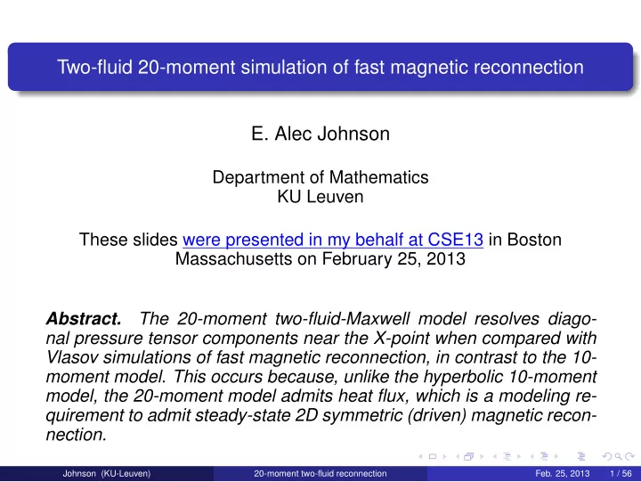
The GEM problem initiates reconnection by pinching adjacent oppositely directed field lines. Two-fluid simulations suggest qualitative agreement with kinetic simulations: Vlasov-Darwin simulations: [SchmitzGrauer06] 5-moment two-fluid-Maxwell simulations: [HaLoSh06], [LoHaSh11]. 10-moment two-fluid-Maxwell simulations: [Hakim06], [JoRo10], [Jo11]. 20-moment two-fluid-Maxwell simulations: [see the following slides]

3718 BIRN ET AL.' GEM RECONNECTION CHALLENGE

X

4 3 2

Full Particle

Hyb rid

Hall MHD

MHD /

I

10 20 30 40

t

Figure 1. The reconnected magnetic flux versus time from a variety of simulation models: full particle, hybrid, Hall MHD, and MHD (for resistivity r/-0.005). phase speed is the factor which limits the electron

ut-

flow velocity from the inner dissipation region (where the electron frozen-in condition is broken) the electron

utflow velocity should

scale like the whistler speed based

n the electron

skin depth. This corresponds to

the electron Alfv•n speed vAe = v/B2/4•men. With

decreasing electron mass the outflow velocity

f elec-

trons should

increase. This trend has

been clearly iden-

tified in particle simulations [Hesse et al., 1999; Hesse et al., this issue; Pritchett, this issue]. A series

f sim-

ulations in the hybrid model confirmed the scaling

f

the outflow velocity with vAe and that the width of the

region

f

high

utflow

velocity scales with c/v:pe [Shay et al., this issue]. The flux of electrons from the inner

dissipation region is therefore independent

f the elec-

tron mass, consistent with the general whistler scaling

argument.

As noted previously, excess dissipation in the Hall

MHD models reduces the reconnection rate below the

large values seen in particle models. On the other hand, large values

f the resistivity

are required in the simulations to prevent the collapse

f the current layers

to the grid scale. The reason is linked to the dispersion properties

f whistler, which controls

the dynamics at

small scale. Including resistivity r/= m•i/ne 2,

Even as k --> cx•, the dissipation term remains small compared with the real frequency as long as There is no scale at which dissipation dominates prop-

agation. The consequence

is that current layers be- come singular unless the resistivity becomes excessive,

even when electron inertia is retained. The resolution

f the problem is straightforward. Dissipation

in the magnetic field equation proportional to V p with p _) 4 can be adjusted to cut in sharply around the grid scale and not strongly diffuse the longer scale lengths which drive reconnection. Such dissipation models are therefore preferable to resistivity in modeling magnetic reconnection with hybrid and Hall MHD codes. The key conclusion

f this project

is that the Hall

effect is the critical factor which must be included to

model collisionless magnetic reconnection. When the Hall physics is included the reconnection rate is fast, corresponding to a reconnection electric field in excess

f 0.2Bov•/c. For typical

parameters

f the plasma

sheet (n .• 0.3cm

3 and

B -• 20 nT), this rate yields

electric fields

f order

4 mV/m. Several caveats must, however, be made before drawing the conclusion that

a Hall MHD or Hall MHD code would be adequate to

model the full dynamics

f the magnetosphere.

The conclusions

f this study pertain explicitly to the 2-D
system. There is mounting

evidence that the narrow layers which develop during reconnection in the 2-D model are strongly unstable to a variety of modes in the full 3-D system. Whether the Hall MHD model provides an adequate description

f these

instabilities and whether these instabilities play a prominent and critical role in triggering reconnection and the onset

f

substorms continues to be debated.

Acknowledgments. This work was supported in part by the NSF and NASA. Janet G. Luhmann thanks

J. D.

Huba and another referee for their assistance in evaluating this paper. References Birn, J., and M. Hesse, Geospace Environmental Modeling (GEM) magnetic reconnection challenge' Resistive tear-

Johnson (KU-Leuven) 20-moment two-fluid reconnection

Feb. 25, 2013

24 / 56

SLIDE 25

Simulation parameters

Symmetry is enforced and system is solved on a quarter-domain for all simulations. All fluid simulations use a 32x64 computational mesh. 3rd-order Runge-Kutta discontinuous Galerkin time scale is ion gyroperiod. Alfv´ en speed is nondimensionalized to 1. so spatial scale is ion skin depth. light speed is 20. relaxation period is chosen to be τs = 50√det Θs/ρs. simulations were run until they crashed on negative pressure (positivity limiting not yet implemented).

Johnson (KU-Leuven) 20-moment two-fluid reconnection

Feb. 25, 2013

25 / 56

SLIDE 26

Reconnecting flux for 10-moment model

Johnson (KU-Leuven) 20-moment two-fluid reconnection

Feb. 25, 2013

26 / 56

SLIDE 27

Reconnecting flux for 10-moment model (again)

Johnson (KU-Leuven) 20-moment two-fluid reconnection

Feb. 25, 2013

27 / 56

SLIDE 28

Reconnecting flux for 20-moment model

Johnson (KU-Leuven) 20-moment two-fluid reconnection

Feb. 25, 2013

28 / 56

SLIDE 29

Johnson (KU-Leuven) 20-moment two-fluid reconnection

Feb. 25, 2013

29 / 56

SLIDE 30

Johnson (KU-Leuven) 20-moment two-fluid reconnection

Feb. 25, 2013

30 / 56

SLIDE 31

Johnson (KU-Leuven) 20-moment two-fluid reconnection

Feb. 25, 2013

31 / 56

SLIDE 32

Johnson (KU-Leuven) 20-moment two-fluid reconnection

Feb. 25, 2013

32 / 56

SLIDE 33

Johnson (KU-Leuven) 20-moment two-fluid reconnection

Feb. 25, 2013

33 / 56

SLIDE 34

Johnson (KU-Leuven) 20-moment two-fluid reconnection

Feb. 25, 2013

34 / 56

SLIDE 35

Johnson (KU-Leuven) 20-moment two-fluid reconnection

Feb. 25, 2013

35 / 56

SLIDE 36

Johnson (KU-Leuven) 20-moment two-fluid reconnection

Feb. 25, 2013

36 / 56

SLIDE 37

Johnson (KU-Leuven) 20-moment two-fluid reconnection

Feb. 25, 2013

37 / 56

SLIDE 38

Johnson (KU-Leuven) 20-moment two-fluid reconnection

Feb. 25, 2013

38 / 56

SLIDE 39

Johnson (KU-Leuven) 20-moment two-fluid reconnection

Feb. 25, 2013

39 / 56

SLIDE 40

Johnson (KU-Leuven) 20-moment two-fluid reconnection

Feb. 25, 2013

40 / 56

SLIDE 41

Johnson (KU-Leuven) 20-moment two-fluid reconnection

Feb. 25, 2013

41 / 56

SLIDE 42

Johnson (KU-Leuven) 20-moment two-fluid reconnection

Feb. 25, 2013

42 / 56

SLIDE 43

Johnson (KU-Leuven) 20-moment two-fluid reconnection

Feb. 25, 2013

43 / 56

SLIDE 44

Johnson (KU-Leuven) 20-moment two-fluid reconnection

Feb. 25, 2013

44 / 56

SLIDE 45

Johnson (KU-Leuven) 20-moment two-fluid reconnection

Feb. 25, 2013

45 / 56

SLIDE 46

Johnson (KU-Leuven) 20-moment two-fluid reconnection

Feb. 25, 2013

46 / 56

SLIDE 47

Johnson (KU-Leuven) 20-moment two-fluid reconnection

Feb. 25, 2013

47 / 56

SLIDE 48

Johnson (KU-Leuven) 20-moment two-fluid reconnection

Feb. 25, 2013

48 / 56

SLIDE 49

Johnson (KU-Leuven) 20-moment two-fluid reconnection

Feb. 25, 2013

49 / 56

SLIDE 50

Off-diagonal components of electron pressure tensor

The 10-moment model resolves off-diagonal pressure tensor components well, because it admits viscous stress. Off-diagonal components of the electron pressure tensor for 10-moment simulation at Ωit = 18 Off-diagonal components of the electron pressure tensor for Vlasov simulation at Ωit = 17.7 [Schmitz- Grauer06]

Johnson (KU-Leuven) 20-moment two-fluid reconnection

Feb. 25, 2013

50 / 56

SLIDE 51

Off-diagonal components of electron pressure tensor

The 20-moment model better resolves the off-diagonal components of the pressure tensor. Off-diagonal components of the electron pressure tensor for 20-moment simulation at Ωit = 16 Off-diagonal components of the electron pressure tensor for Vlasov simulation at Ωit = 17.7 [Schmitz- Grauer06]

Johnson (KU-Leuven) 20-moment two-fluid reconnection

Feb. 25, 2013

51 / 56

SLIDE 52

Diagonal components of electron pressure tensor

The 10-moment model resolves the diagonal components of the pressure tensor near the X-point poorly, because it does not admit heat flux. Diagonal components of the electron pressure tensor for 10-moment simulation at Ωit = 18 Diagonal components of the electron pressure tensor for Vlasov simulation at Ωit = 17.7 [SchmitzGrauer06]

Johnson (KU-Leuven) 20-moment two-fluid reconnection

Feb. 25, 2013

52 / 56

SLIDE 53

Diagonal components of electron pressure tensor

The 20-moment model resolves the diagonal components of the pressure tensor near the X-point better, because it admits heat flux. Diagonal components of the electron pressure tensor for 20-moment simulation at Ωit = 16 Diagonal components of the electron pressure tensor for Vlasov simulation at Ωit = 17.7 [SchmitzGrauer06]

Johnson (KU-Leuven) 20-moment two-fluid reconnection

Feb. 25, 2013

53 / 56

SLIDE 54

Requirements for steady 2D symmetric magnetic reconnection

Consider the simplest reconnection scenario: steady 2D reconnection symmetric under 180-degree rotation about the X-point.

Theorem

Reconnection is impossible without viscosity or resistivity. Argument: Rate of reconnection is the electric field strength at the X-point. Electric field strength at the X-point is resistive electric field plus viscous electric field.

Theorem (Jo11)

Reconnection is impossible for any conservative model for which heat flux is zero. Argument: Steady reconnection requires entropy production near the X-point (via resistivity or viscosity). The X-point is a stagnation point. Without heat flux, heat accumulates at the X-point without bound. Observation: in kinetic simulations, fast reconnection is supported by viscosity, not resistivity. Conclusion: we need heat flux and viscosity in a fluid model of fast magnetic reconnection.

Johnson (KU-Leuven) 20-moment two-fluid reconnection

Feb. 25, 2013

54 / 56

SLIDE 55

Performance summary of fluid models

Performance of hyperbolic fluid models relative to kinetic simulations: 5-moment

Success: rate of reconnection is qualitatively correct. Reason for success: reconnection wants to happen, and the inertial term provides a mechanism. Failure: reconnection is supported by inertial term rather than pressure term. Reason for failure: lack of viscosity forces current to ramp at the X-point until mitigated by numerical

resistivity. [Jo11]

10-moment [Jo11]:

Success: pressure tensor supports reconnection

model shows reasonable resolution of off-diagonal components of electron pressure tensor. [JoRo10]. reconnection is insensitive to collision period τs reconnection is robust and reliable if τs = ∞ is used to damp oscillations in deviatoric stress [Jo11]

Reason for success: the model admits viscosity. Failure: diagonal components of pressure tensor are poorly resolved near X-point Reason for failure: lack of heat flux forces entropy and pressure anisotropy to ramp at the X-point. Instability eventually kicks in. [Jo11]

20-moment:

Success: diagonal components of electron pressure tensor are resolved near X-point. Reason for success: the model admits heat flux to relieve temperature pile-up. Issue: need for positivity limiting and instability are seen at late times. What to do about it:

A generic framework for positivity limiting is developed in [JoRo13]. The GEM problem is unstable to secondary plasmoid formation, so convergence becomes unfeasible for any accurate model at late times. For stable steady reconnection an implicit method is called for.

Johnson (KU-Leuven) 20-moment two-fluid reconnection

Feb. 25, 2013

55 / 56

SLIDE 56

References

[Brown96] Shawn Lee Brown. Approximate Riemann solvers for moment models of dilute gases. PhD thesis, University of Michigan (1996). [GEM01] J. Birn, J. Drake, M. Shay, B. Rogers, R. Denton, M. Hesse, M. Kuznetsova, Z. Ma, A. Bhattacharjee, A. Otto, and P .

Pritchett. Geospace environmental modeling (GEM) magnetic reconnection challenge. Journal of Geophysical Research —

Space Physics, 106:3715–3719, 2001. [GrothGRB94] Clinton P . T. Groth, Tamas I. Gombosi, Philip L. Roe, and Shawn L. Brown, Gaussian-based moment-method closures for the solution of the Boltzmann equation. Proceedings of the Fifth International Conference on Hyperbolic Problems. Theory, Numerics, Applications. University of New York at Stony Brook, Stony Brook, New York, USA, 1994, World Scientific, New Jersey, pp. 339–346. [Grad49] Harold Grad. On the Kinetic Theory of Rarefied Gases. Commun. Pure Appl. Math., Vol. 2, pp. 331–407. [GrothGRB03] C.P .T. Groth, T.I. Gombosi, P .L. Roe, and S.L. Brown. A Gaussian-based closure for rarefied gases: derivation, moment equations, and wave structure. Unpublished paper written in 2003 and obtained from Groth. [Hakim06] A. Hakim. Extended MHD modelling with the ten-moment equations. Journal of Fusion Energy, 27 (2008). [HaLoSh06] A. Hakim, J. Loverich, and U. Shumlak. A high-resolution wave propagation scheme for ideal two-fluid plasma

equations. J. Comp. Phys., 219 (2006), pp. 418–442.

[Jo11] E.A. Johnson, Gaussian-Moment Relaxation Closures for Verifiable Numerical Simulation of Fast Magnetic Reconnection in

Plasma. PhD thesis, UW–Madison, 2011

[JoRo10] E. A. Johnson and J. A. Rossmanith, Ten-moment two-fluid plasma model agrees well with PIC/Vlasov in GEM problem. ‘proceedings for HYP2010, November 2010. [JoRo13] E. A. Johnson and J. A. Rossmanith, Outflow Positivity Limiting for Hyperbolic Conservation Laws. Part I: Framework and

Recipe. http://arxiv.org/abs/1212.4695.

[LoHaSh11] J. Loverich, A. Hakim, and U. Shumlak A discontinuous Galerkin method for ideal two-fluid plasma equations. Commun.

Comput. Phys., 9 (2011), pp. 240–268.

[SchmitzGrauer06] H. Schmitz and R. Grauer. Darwin-Vlasov simulations of magnetised plasmas. J. Comp. Phys., 214 (2006), pp. 738–756.

Johnson (KU-Leuven) 20-moment two-fluid reconnection

Feb. 25, 2013

56 / 56