Turing machine (Alan Turing 1936) CS 3813: Introduction to Formal - - PDF document

1

CS 3813: Introduction to Formal Languages and Automata

Turing machines (9.1)

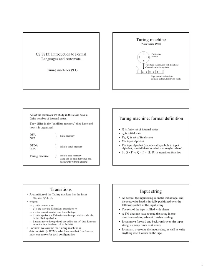
Turing machine

(Alan Turing 1936) 1 2 3 a a b a b

Finite-state control Tape head can move in both directions Can read and write symbols Tape extends infinitely to the right and left, filled with blanks

All of the automata we study in this class have a finite number of internal states. They differ in the “auxiliary memory” they have and how it is organized. DFA NFA DPDA PDA Turing machine

finite memory infinite stack memory infinite tape memory (tape can be read forwards and backwards without erasing)

Turing machine: formal definition

• Q is finite set of internal states
• q0 is initial state
• F ⊆ Q is set of final states
• Σ is input alphabet
• Γ is tape alphabet (includes all symbols in input

alphabet, special blank symbol, and maybe others)

• δ : Q × Γ → Q × Γ × {L, R} is transition function

Transitions

• A transition of the Turing machine has the form

δ(q, a) = (q’, b, L),

• where:

– q is the current state, – q’ is the state the TM makes a transition to, – a is the current symbol read from the tape, – b is the symbol the TM writes on the tape, which could also be the blank symbol, ♦ – L means move the tape head one cell to the left (and R means move the tape head one cell to the left)

• For now, we assume the Turing machine is

deterministic (a DTM), which means that δ defines at most one move for each configuration

Input string

• As before, the input string is on the initial tape, and

the read/write head is initially positioned over the leftmost symbol of the input string

• The rest of the tape is filled with blanks
• A TM does not have to read the string in one

direction and stop when it finishes reading

• It can move forward and backwards over the input

string, as many times as it wants

• It can also overwrite the input string, as well as write

anything else it wants on the tape

2

Halting

• When does a TM halt?

– when it reaches a configuration for which there is no transition defined – when it enters a final state (we will assume no transitions are defined for a final state)

• It is important to note that a TM does not

necessarily halt. It can enter an infinite loop.

Acceptance

• We can define how a TM accepts a string in

different ways.

• We will say that it accepts a string if it halts in

final state. It rejects the string if it halts in some other state, or does not halt at all.

Example

The following diagram represents a TM that accepts the language denoted by the regular expression a*b*.

a → a,R b → b,R b → b,R ♦ → ♦,L

q0 q1 q2

How do you write the transitions for this?

♦ → ♦,L

Exercises

• Recall that the following languages are not

context-free. – {anbncn|n ≥ 0} – {ww | w ∈ {a,b}*}

• In English, describe how a Turing machine

could accept each of these languages

• Try to draw the transition diagrams for the

Turing machines

Model of computation

• A TM is an abstract model of a computer

that lets us define in a precise, mathematical way what we mean by computation.

• As before, we use the concept of a

“configuration” to define what we mean by computation.

Configuration

• A configuration of a TM includes everything

we need to know to continue a computation

– current state – symbol currently under the tape head – string on tape to left of the head (up to leftmost non

• b

lank symbol) – string on tape to right of the head (up to rightmost non

• b

l ank symbol)

• Example

– (q, a, abb, bbb)

3

Computation

• A computation is a sequence of

configurations such that each configuration is obtained from the previous configuration by some transition of the TM

Computing functions

• We use automata to recognize languages and

compute functions (although we haven’t talked about computing functions until now).

• In fact, computing functions allows language

recognition, since every language can be represented by a characteristic function

– if the input string is in the language, output 1 – otherwise output 0

String and numeric functions

• A TM can compute functions on strings. Given an

input string, the output of the function is the string left

• n the tape after the TM halts.
• A TM can also compute numeric functions. Using a

binary alphabet for strings, the input string can represent a binary number and the output string can represent a binary number. (A unary alphabet can also be used, as in the book.)

• A TM can compute a function with multiple
• arguments. Each argument is separated by a special

character, delimiter, on the tape.

Transducers

• We can create TMs that compute arithmetic

functions such as addition, subtraction, multiplication, etc.

• A TM that computes other things besides

language acceptance is called a transducer. A transducer computers some output (which could be anything) for some input.

Exercise

Construct (or describe how to construct) a TM that computes the numeric function f(k) = k + 1.