SLIDE 1
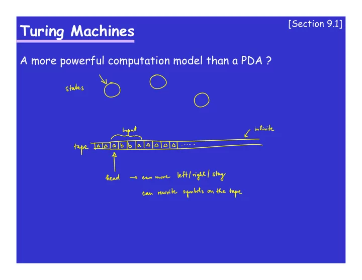
Turing Machines
A more powerful computation model than a PDA ?
[Section 9.1]
SLIDE 2 Turing Machines
Some history:
- introduced by Alan Turing in 1936
- models a “human computer”
(human writes/rewrites symbols on a sheet of paper, the human’s state of mind changes based on what s/he has seen)
- a reasonable model for real computers
Church-Turing Thesis: For any problem L (given by a language) there exists an algorithm iff there exists a Turing machine which terminates
[Section 9.1]
SLIDE 3
Real-world problems vs. languages
Example : the airline problem - given are airports and available flights, is it possible to get from a place A to a place B ?
[Section 9.1]
SLIDE 4 [Section 9.1]
Verbal explanation:
- The tape is infinite to the right and it initially contains the
input string (the rest of the tape contains blanks - M).
- The TM starts in an initial state, reading the first symbol on
the tape.
- The head can move left, right, or stay at its current position.
- The TM has two special states, ha (accept) and hr (reject).
- If the head moves to the left of the first symbol, this
automatically means the change of state to hr (reject).
- The transition is specified by a state and a tape symbol (to
which the head points). It returns a new state, new tape symbol (to rewrite the original), and a head-move (L/R/S).
Turing Machines cont.
SLIDE 5
Turing Machines cont.
[Section 9.1]
Example : As a warm-up, give a Turing machine for a*b*c* Simplified transition diagram : we do not have to draw transitions leading to hr.
SLIDE 6 [Section 9.1]
A Turing machine (TM) is a 5-tuple (Q,Σ,Γ,q0,δ) where
- Q is a finite set of states not containing ha, hr (the two
halting states)
is a finite alphabet (input symbols)
is a finite alphabet (tape symbols) such that Σ ⊆ Γ and Γ does not contain M (the blank symbol)
- qo ∈ Q is the initial state
- δ : ___________ → _______________________
is a partial function defining the transitions
Turing Machines cont.
SLIDE 7
[Section 9.1]
Let T = (Q,Σ,Γ,q0,δ) be a TM. A configuration of T is ________________. The initial configuration is ________________. We use `T to say that T can get from one configuration to another configuration using a single transition. We use `T
* to say that T can get from one configuration to
another configuration using a sequence of transitions.
Turing Machines cont.
SLIDE 8 [Section 9.1]
Let T = (Q,Σ,Γ,q0,δ) be a TM and x ∈ Σ*. We say that x is accepted by T if _____________________ . The language accepted by T, denoted L(T), is the set of all strings in Σ* that are accepted by T. A string x can be rejected in two ways : either the computation of T on x ends in the state hr, or the computation
- f T on x gets into an infinite loop.
A language accepted by a TM is called recursively enumerable. A language for which there is a TM which never goes to an infinite loop is called recursive.
Turing Machines cont.
SLIDE 9
[Section 9.1]
Example: Give a TM accepting { akbkck | k ≥ 0 }.
Turing Machines cont.
SLIDE 10
[Section 9.2]
Let T = (Q,Σ,Γ,q0,δ) be a TM and let f be a total function from Σ* to Γ*. We say that T computes f if for every x ∈ Σ*, (q0, Mx) `T
* (ha, Mf(x)).
Example : give a TM that computes the function f(1n) = 12n
Turing Machines and functions
SLIDE 11 [Section 9.4]
Possible attempts to make Turing machines stronger :
- 2-way infinite tape
- several heads, several tapes
- random access (the head can jump to any position)
- nondeterminism
- etc.
Note: All of the above changes can be simulated by a TM.
A stronger machine than a TM ?
SLIDE 12
[Section 9.4]
Example : How to simulate a 2-way infinite tape using a regular TM ?
A stronger machine than a TM ?
SLIDE 13
[Section 9.5]
The definition is the same as Turing machines, except that the transition function goes from Q × (Γ ∪ {M}) to subsets of (Q ∪ {ha,hr}) × (Γ ∪ {M}) × {R,L,S}. Thm : Let T1 be an NTM. Then there exist a TM T2 such that L(T1)=L(T2).
Nondeterministic TM (NTM)