truss like mixed mode cohesive laws is independent 0 0 of
play

truss-like mixed mode cohesive laws is independent 0 0 of the - PDF document

18 TH INTERNATIONAL CONFERENCE ON COMPOSITE MATERIALS WORK OF SEPARATION OF TRUSS-LIKE MIXED MODE COHESIVE LAWS S. Goutianos, B. F. Srensen* Materials Research Division, Ris National Laboratory for Sustainable Energy, Technical University of


  1. 18 TH INTERNATIONAL CONFERENCE ON COMPOSITE MATERIALS WORK OF SEPARATION OF TRUSS-LIKE MIXED MODE COHESIVE LAWS S. Goutianos, B. F. Sørensen* Materials Research Division, Risø National Laboratory for Sustainable Energy, Technical University of Denmark, DK-4000 Roskilde, Denmark author( bsqr@risoe.dtu.dk ) Keywords : mixed mode cohesive law; cohesive element; path dependence 
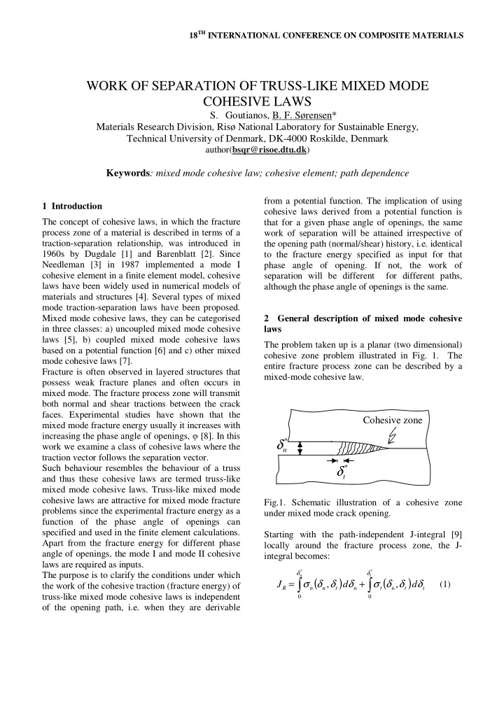
from a potential function. The implication of using 1 Introduction cohesive laws derived from a potential function is The concept of cohesive laws, in which the fracture that for a given phase angle of openings, the same process zone of a material is described in terms of a work of separation will be attained irrespective of traction-separation relationship, was introduced in the opening path (normal/shear) history, i.e. identical 1960s by Dugdale [1] and Barenblatt [2]. Since to the fracture energy specified as input for that Needleman [3] in 1987 implemented a mode I phase angle of opening. If not, the work of cohesive element in a finite element model, cohesive separation will be different for different paths, laws have been widely used in numerical models of although the phase angle of openings is the same. materials and structures [4]. Several types of mixed mode traction-separation laws have been proposed. Mixed mode cohesive laws, they can be categorised 2 General description of mixed mode cohesive in three classes: a) uncoupled mixed mode cohesive laws laws [5], b) coupled mixed mode cohesive laws The problem taken up is a planar (two dimensional) based on a potential function [6] and c) other mixed cohesive zone problem illustrated in Fig. 1. The mode cohesive laws [7]. entire fracture process zone can be described by a Fracture is often observed in layered structures that mixed-mode cohesive law. possess weak fracture planes and often occurs in mixed mode. The fracture process zone will transmit both normal and shear tractions between the crack faces. Experimental studies have shown that the Cohesive zone mixed mode fracture energy usually it increases with increasing the phase angle of openings, φ [8]. In this * δ work we examine a class of cohesive laws where the n traction vector follows the separation vector. Such behaviour resembles the behaviour of a truss * δ t and thus these cohesive laws are termed truss-like mixed mode cohesive laws. Truss-like mixed mode cohesive laws are attractive for mixed mode fracture Fig.1. Schematic illustration of a cohesive zone problems since the experimental fracture energy as a under mixed mode crack opening. function of the phase angle of openings can specified and used in the finite element calculations. Starting with the path-independent J-integral [9] Apart from the fracture energy for different phase locally around the fracture process zone, the J- angle of openings, the mode I and mode II cohesive integral becomes: laws are required as inputs. * * δ δ The purpose is to clarify the conditions under which n t ( ) ( ) = σ δ , δ δ + σ δ , δ δ J d d (1) the work of the cohesive traction (fracture energy) of R n n t n t n t t ∫ ∫ truss-like mixed mode cohesive laws is independent 0 0 of the opening path, i.e. when they are derivable

  2. The end-openings δ * n and δ * where σ n and σ t are the normal and shear tractions, t (Cartesian form) can be δ n and δ t the normal and tangential crack opening transformed to polar form: displacements, δ * n and δ * t the normal and tangential * δ crack opening displacements at the end of the 2 2 * * * * − 1 t δ = δ + δ , ϕ = tan   (7) m n t * cohesive zone as indicated in Fig. 1.   δ   n The J integral result (Eq. 1) can be interpreted as the   where δ * m is the end-opening magnitude and φ * its work (per unit fracture area) of the cohesive tractions at the end of the cohesive zone. This holds phase angle of openings. Then the cohesive tractions for any values of δ * n and δ * t . J R defined according to (Eqs, 5 and 6) can be written as [10]: Eq. 1 is called the fracture resistance. When the cohesive zone is fully developed δ * n = δ f n and δ * t = δ f t ), * ∂ J sin ϕ ∂ J J R equals the work of separation, also called the * * σ = ϕ R − R cos (8) n fracture energy. δ f n and δ f * * * t are the critical normal and ∂ δ δ ∂ ϕ m m tangential openings for complete failure (the corresponding tractions are equal to zero). * ∂ cos ϕ ∂ J J If it is assumed that the tractions are derived from a * * σ = ϕ R − R sin (9) t * * * potential function, Φ , then the normal σ n , and shear ∂ δ δ ∂ ϕ m m σ t tractions can be taken to be functions of both δ n and δ t but independent of position within the cohesive zone: 3 Truss-like cohesive laws ∂ Φ ( δ , δ ) n t As mentioned in the Introduction, for truss-like σ ( δ , δ ) = (2) n n t ∂ δ cohesive laws the phase angle of the cohesive n traction vector, ψ , and the phase angle of the openings, φ , must be identical for any point within ∂ Φ δ δ ( , ) σ ( δ , δ ) = n t the cohesive zone, ψ = φ . This also holds for the end- (3) t n t ∂ δ openings. Thus, the direction of cohesive tractions at t the end of the cohesive zone must follow the From Eqs. 1, 2 and 2, the J integral becomes: direction of the end-openings: * * = Φ ( δ , δ ) J (4) * * ψ = ϕ (10) R n t Finally, from Eqs. 2, 3 and 4, the following where the phase angle of the traction vector at the expressions for the cohesive tractions at the end of end of the cohesive zone is: the cohesive zone can be obtained: * σ * − 1 * * t ∂ δ δ ψ = tan   J ( , ) (11) * * * R n t * σ = σ ( δ , δ ) =   (5) σ   n n n t * n ∂ δ   n Then, by substituting Eqs. 8 and 9 into Eq. 11 it can be shown that [10]: * * ∂ J ( δ , δ ) * * * σ = σ ( δ , δ ) = R n t (6) t t n t * ∂ J ∂ δ R * = 0 t (12) ∂ ϕ In Eqs 5 and 6 an asterix indicates the position of the end of the cohesive zone. However, since the This implies that when ψ * = φ * (truss-like cohesive cohesive laws are assumed to be the same at any laws) the tractions can be derived from a potential position within the cohesive zone, the cohesive laws function only when J R is independent of the phase at the end-openings (Eqs. 5 and 6) must be identical angle of the openings. Note that it is the fracture to the cohesive law at any position within the resistance, J R , defined from Eq. 1, not just the cohesive zone. fracture energy (the work of separation), that must

  3. be independent of φ * for the tractions to be derivable If the cohesive tractions for truss-like mixed mode from a potential function. cohesive laws with linear softening can be derived from a potential function, they must fulfill the following condition [11]: 4 Truss-like mixed mode cohesive laws with linear softening ∂ σ ∂ σ n = t A type of widely used truss-like mixed mode bi- (16) ∂ δ ∂ δ linear cohesive laws is used to verify the general t n result of Eq. 12. Fig. 2 shows a sketch of the It can be shown that when the cohesive tractions are bilinear cohesive laws for pure mode I and pure described by Eqs. 13 and 14, the criterion given in ⌢ and σ mode II used here. The mode I peak stress is Eq. 16 is satisfied only when the fracture resistance, n ⌢ . The corresponding J R , is independent of the phase angle of openings. σ the mode II peak stress is t o o δ and δ . openings are n t In the linear softening part the tractions are given by: 5 Numerical verification The analytical results presented above are verified σ ( δ ) = ( 1 − ) δ D K (13) n n n n numerically by the commercial finite element code Abaqus. In order to check the path dependence of σ ( δ ) = ( 1 − ) δ D K (14) the truss-like bi-linear cohesive laws described in t t t t Section 4, three opening paths are chosen to the It can be shown that when ψ = φ , the damage variable same normal and tangential separations as shown in D is [10]: Fig. 3. If the mixed mode cohesive law is path independent, the work of cohesive tractions should be the same for the three different opening paths. f o f o δ ( δ − δ cos ϕ ) δ ( δ − δ sin ϕ ) = m n m = m t m D (15) f o f o δ − δ δ δ − δ δ ( ) ( ) m m t m m t where δ o m and δ f m are the mixed-mode critical + opening for crack initiation and opening at complete a failure, respectively. c b + Fig.3. Different loading paths (displacement controlled): a) Normal opening, followed by tangential opening, Γ n → t , b) Tangential opening Fig.2. Schematic illustration of bilinear traction- followed by normal opening, Γ t → n , and c) separation laws (normal and tangential directions). proportional loading, Γ p . 3

Download Presentation
Download Policy: The content available on the website is offered to you 'AS IS' for your personal information and use only. It cannot be commercialized, licensed, or distributed on other websites without prior consent from the author. To download a presentation, simply click this link. If you encounter any difficulties during the download process, it's possible that the publisher has removed the file from their server.

Recommend


More recommend