Topics for today Introduction to R Graphics: Getting started with - PowerPoint PPT Presentation

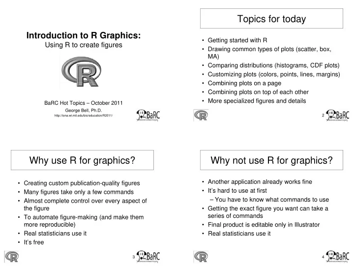
Topics for today Introduction to R Graphics: • Getting started with R g U i R t t fi Using R to create figures • Drawing common types of plots (scatter, box, MA) • Comparing distributions (histograms, CDF plots) • Customizing plots (colors, points, lines, margins) • Combining plots on a page • Combining plots on a page • Combining plots on top of each other • More specialized figures and details BaRC Hot Topics – October 2011 George Bell, Ph.D. http://iona.wi.mit.edu/bio/education/R2011/ 2 Why use R for graphics? Why not use R for graphics? • Another application already works fine pp y • Creating custom publication-quality figures Creating custom publication quality figures • It’s hard to use at first • Many figures take only a few commands – You have to know what commands to use • Almost complete control over every aspect of the figure • Getting the exact figure you want can take a series of commands • To automate figure-making (and make them more reproducible) more reproducible) • Final product is editable only in Illustrator • Final product is editable only in Illustrator • Real statisticians use it • Real statisticians use it • It’s free 3 4

Getting started Start of an R session On tak On your own computer • See previous session: Introduction to R: See previous session: Introduction to R: http://iona.wi.mit.edu/bio/education/R2011/ • Hot Topics slides: http://iona.wi.mit.edu/bio/hot_topics/ • R can be run on your computer or on tak. 5 6 Getting help Reading files - intro • Use the Help menu • Take R to your preferred directory () • Check out “Manuals” • Check out Manuals Html help – http://www.r-project.org/ – contributed documentation • Use R’s help ?boxplot [show info] ??boxplot [search docs] • Check where you are (e.g., get your working directory) y ( g , g y g y) example(boxplot) [examples] and see what files are there • Search the web > getwd() [1] "X:/bell/Hot_Topics/Intro_to_R“ – “r-project boxplot” > dir() [1] “all_my_data.txt" 7 8

Reading data files Figure formats and sizes • By default, a figure window will pop up from most R sessions. • Usually it’s easiest to read data from a file • Instead, helpful figure names can be included in code – Pro: You won t need an extra step to save the figure Pro: You won’t need an extra step to save the figure – Organize in Excel with one-word column names Organize in Excel with one word column names – Con: You won’t see what you’re creating – Save as tab-delimited text • To select name and size (in inches) of pdf file (which can be >1 page) • Check that file is there pdf(“tumor_boxplot.pdf”, w=11, h=8.5) boxplot(tumors) # can have >1 page dev.off() # tell R that we’re done list.files() • To create another format (with size in pixels) • Read file png(“tumor_boxplot.png”, w=1800, h=1200) boxplot(tumors) tumors = read.delim( tumors_wt_ko.txt , header=T) tumors = read delim("tumors wt ko txt" header=T) dev.off() • Check that it’s OK • Save your commands (in a text file)! > tumors • Final PDF figures wt ko – can be converted with Acrobat 1 5 8 – are be edited with Illustrator 2 6 9 3 7 11 9 10 Introduction to scatterplots Boxplot conventions • Simplest use of the ‘plot’ command wt ko • Can draw any number of points C d b f i t 5 8 6 9 • Example (comparison of expression values) <= 1.5 x IQR 75 th percentile 7 11 genes = read.delim(“Gene_exp_with_sd.txt”) IQR = interquartile range median plot(genes$WT, genes$KO) Gene WT KO 25 th percentile Any points A 6 8 beyond the whiskers are B 5 5 defined as defined as C 9 12 “outliers”. Right-click to save figure D 4 5 Note that the E 8 9 above data has no F 6 8 “outliers”. The red point was added by But note that A = F 11 hand. 12 Other programs use different conventions!

Comparing sets of numbers Gene expression plots • Why are you making the figure? Typical x-y scatterplot MA (ratio-intensity) plot x-y scatterplot with contour • What is it supposed to show? pp • How much detail is best? • Are the data points paired? plot(genes.all) M = genes.all[,2] - genes.all[,1] library(MASS) abline(0,1) A = apply(genes.all, 1, mean) kde2d() # et density # Add other lines plot(A,M) image() # Draw colors # etc. contour() # Add contour plot(genes) stripchart(genes, vert=T) boxplot(genes) points() # Add points Note the “jitter” (addition of noise) in the first 2 figures. 13 14 Comparing distributions Displaying distributions • Example dataset: log2 expression ratios • Why are you making the figure? • What is it supposed to show? • How much detail is best? • Methods: – Boxplot – Histogram – Density plot – Violin plot – CDF (cumulative distribution function) plot 15 16

Comparing similar distributions Customizing plots • About anything about a plot can be modified, Density plot • Example dataset: • Example dataset: although it can be tricky to figure out how to do although it can be tricky to figure out how to do – MicroRNA is knocked so. down – Colors ex: col=“red” – Expression levels are – Shapes of points ex: pch=18 assayed – Shapes of lines ex: lwd=3, lty=3 CDF plot – Genes are divided into – Axes (labels scale orientation size) Axes (labels, scale, orientation, size) those without miRNA – Margins see ‘mai’ in par() target site (black) vs. – Additional text ex: text(2, 3, “This text”) with target site (red) – See par() for a lot more options 17 18 Point shapes by number Customizing a plot • plot(x, y, type="p") • plot(x, y, type="p", pch=21, col="black", bg=rainbow(6), cex=x+1, ylim=c(0, max(c(y1,y2))), xlab="Time (d)", ylab="Tumor counts", las=1, Ex: cex.axis=1.5, cex.lab=1.5, main="Customized figure", cex.main=1.5) pch=21 • Non-obvious options: – type="p“ yp p # Draw points p – pch=21 # Draw a 2-color circle – col="black“ # Outside color of points – bg=rainbow(6) # Inside color of points – cex=x+1 # Size points using ‘x’ – las=1 # Print horizontal axis labels 19 20

Combining plots on a page Merging plots on same figure • Set up layout with command like • Commands: – par(mfrow = c(num.rows, num.columns)) par(mfrow c(num rows num columns)) – plot plot # start figure # start figure – Ex: par(mfrow = c(1,2)) – points # add point(s) – lines # add line(s) – legend • Note that order of • Note that order of commands determines order of layers 21 22 More graphics details Using error bars library(plotrix) • Creating error bars plotCI(x, y, uiw=y.sd, liw=y.sd) p ( , y, y , y ) # vertical error bars • Drawing a best-fit (regression) line plotCI(x, y, uiw=x.sd, liw=x.sd, err="x", add=T) # horizontal • Using transparent colors • Creating colored segments • Creating log-transformed axes • Labeling selected points • Labeling selected points 23 24

Drawing a regression line Transparent colors • Use ‘lm(response~terms)’ for simple linear regression: regression: • Semitransparent colors can # Calculate y-intercept be indicated by an lmfit = lm(y ~ x) extended RGB code # Set y-intercept to 0 (#RRGGBBAA) – AA = opacity from 0-9,A-F lmfit.0 = lm(y ~ x + 0) (lowest to highest) • Add line(s) with – Sample colors: Red #FF000066 abline(lmfit) Green #00FF0066 Blue #0000FF66 25 26 Colored bars Handling log tranformations • Data or axes can be transformed or scaled. • Which (if either) should be used? Whi h (if ith ) h ld b d? • Colored bars can be used C l d b b d to label rows or columns of a matrix – Ex: cell types, GO terms • Limit each color code to 6- 8 8 colors l • Don’t forget the legend! 27 28

Labeling selected points More resources • R Graph Gallery: 1. Make figure – http://addictedtor.free.fr/graphiques/ http://addictedtor.free.fr/graphiques/ 2. Run “identify” command • R scripts for Bioinformatics – identify(x, y, – http://iona.wi.mit.edu/bio/bioinfo/Rscripts/ labels) • List of R modules installed on tak – Ex: identify(genes, – http://tak/trac/wiki/R labels = • Our favorite book: rownames(genes)) – Introductory Statistics with R 3 3. Click at or near points Click at or near points (Peter Dalgard) to label them • We’re glad to share commands and/or scripts to get 4. Save image you started WT cells KO cells MUC5B::727897 31.7 41.7 HAPLN4::404037 37.3 47.7 29 30 SIGLEC16::400709 24.1 32.7 Upcoming Hot Topics • Introduction to Bioconductor - microarray and RNA-Seq analysis (Thursday) • Unix, Perl, and Perl modules (short course) • Quality control for high-throughput data • RNA-Seq analysis • Gene list enrichment analysis • Galaxy • Sequence alignment: pairwise and multiple Sequence alignment: pairwise and multiple • See http://iona.wi.mit.edu/bio/hot_topics/ • Other ideas? Let us know. 31