Todays Outline Reinforcement Learning Dan Weld Reinforcement - - PDF document

SLIDE 1

5/7/2012 1

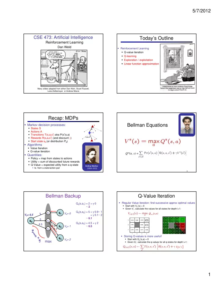
CSE 473: Artificial Intelligence

Reinforcement Learning

Dan Weld

Many slides adapted from either Dan Klein, Stuart Russell, Luke Zettlemoyer or Andrew Moore

1

Today’s Outline

• Reinforcement Learning
• Q-value iteration
• Q-learning
• Exploration / exploitation
• Linear function approximation
• Linear function approximation

Recap: MDPs

• Markov decision processes:
• States S
• Actions A
• Transitions T(s,a,sʼ) aka P(sʼ|s,a)
• Rewards R(s,a,sʼ) (and discount )
• Start state s0 (or distribution P0)

a s s, a s,a,sʼ sʼ

0 ( 0)

• Algorithms
• Value Iteration
• Q-value iteration
• Quantities:
• Policy = map from states to actions
• Utility = sum of discounted future rewards
• Q-Value = expected utility from a q-state
• Ie. from a state/action pair

Andrey Markov (1856‐1922)

Bellman Equations

4

Q*(a, s) =

Bellman Backup

V4= 0 Q5(s,a1) = 2 +  0 ~ 2 Q5(s,a2) = 5 +  0.9~ 1 +  0.1~ 2 ~ 6.1 V5= 6.5 5

a2 a1

s0 s1

V4= 1 V4= 2 Q5(s,a3) = 4.5 +  2 ~ 6.5

max

a2 a3

s0 s2 s3

Q-Value Iteration

• Regular Value iteration: find successive approx optimal values
• Start with V0

*(s) = 0

• Given Vi

*, calculate the values for all states for depth i+1:

Qi+1(s,a)

• Storing Q-values is more useful!
• Start with Q0

*(s,a) = 0

• Given Qi

*, calculate the q-values for all q-states for depth i+1:

Vi(s’) ]

SLIDE 2

5/7/2012 2

Q-Value Iteration

Initialize each q-state: Q0(s,a) = 0 Repeat

For all q-states, s,a Compute Qi+1(s,a) from Qi by Bellman backup at s,a.

Until maxs,a |Qi+1(s,a) – Qi(s,a)| < 

Vi(s’) ]

Reinforcement Learning

• Markov decision processes:
• States S
• Actions A
• Transitions T(s,a,sʼ) aka P(sʼ|s,a)
• Rewards R(s,a,sʼ) (and discount )
• Start state s0 (or distribution P0)

a s s, a s,a,sʼ

0 ( 0)

• Algorithms
• Q-value iteration  Q-learning
• Approaches for mixing exploration & exploitation
• -greedy
• Exploration functions

sʼ

Applications

• Robotic control
• helicopter maneuvering, autonomous vehicles
• Mars rover - path planning, oversubscription planning

g g

• elevator planning
• Game playing - backgammon, tetris, checkers
• Neuroscience
• Computational Finance, Sequential Auctions
• Assisting elderly in simple tasks
• Spoken dialog management
• Communication Networks – switching, routing, flow control
• War planning, evacuation planning

Stanford Autonomous Helicopter

http://heli.stanford.edu/

10

Two main reinforcement learning approaches

• Model-based approaches:
• explore environment & learn model, T=P(sʼ|s,a) and R(s,a),

(almost) everywhere

• use model to plan policy, MDP-style

h l d t t t th ti l lt

• approach leads to strongest theoretical results
• often works well when state-space is manageable
• Model-free approach:
• donʼt learn a model; learn value function or policy directly
• weaker theoretical results
• often works better when state space is large

Two main reinforcement learning approaches

• Model-based approaches:

Learn T + R |S|2|A| + |S||A| parameters (40,000)

• Model-free approach:

Learn Q |S||A| parameters (400)

SLIDE 3

5/7/2012 3

Recap: Sampling Expectations

• Want to compute an expectation weighted by P(x):
• Model-based: estimate P(x) from samples, compute expectation
• Model-free: estimate expectation directly from samples
• Why does this work? Because samples appear with the right

frequencies!

Recap: Exp. Moving Average

• Exponential moving average
• Makes recent samples more important
• Forgets about the past (distant past values were wrong anyway)
• Easy to compute from the running average
• Decreasing learning rate can give converging averages

Q-Learning Update

• Q-Learning = sample-based Q-value iteration
• How learn Q*(s,a) values?
• Receive a sample (s a sʼ r)
• Receive a sample (s,a,s ,r)
• Consider your old estimate:
• Consider your new sample estimate:
• Incorporate the new estimate into a running average:

Exploration-Exploitation tradeoff

• You have visited part of the state space and found a

reward of 100

• is this the best you can hope for???
• Exploitation: should I stick with what I know and find

d li hi k l d ?

16

a good policy w.r.t. this knowledge?

• at risk of missing out on a better reward somewhere
• Exploration: should I look for states w/ more

reward?

• at risk of wasting time & getting some negative reward

Exploration / Exploitation

• Several schemes for action selection
• Simplest: random actions ( greedy)
• Every time step, flip a coin
• With probability  , act randomly

With b bilit 1 t di t t li

• Problems with random actions?
• You do explore the space, but keep thrashing

around once learning is done

• One solution: lower  over time
• Another solution: exploration functions
• With probability 1- , act according to current policy

Q-Learning:  Greedy

QuickTime™ and a H.264 decompressor are needed to see this picture.

SLIDE 4

5/7/2012 4

Exploration Functions

• Exploration function
• When to explore
• Random actions: explore a fixed amount
• Better idea: explore areas whose badness is not (yet) established

Exploration function

• Takes a value estimate and a count, and returns an
• ptimistic utility, e.g.

(exact form not important)

• Exploration policy π(s’)=

vs.

Q-Learning Final Solution

• Q-learning produces tables of q-values:

Q-Learning Properties

• Amazing result: Q-learning converges to optimal policy
• If you explore enough
• If you make the learning rate small enough
• … but not decrease it too quickly!
• Not too sensitive to how you select actions (!)

y ( )

• Neat property: off-policy learning
• learn optimal policy without following it (some caveats)

S E S E

Q-Learning – Small Problem

• Doesn’t work
• In realistic situations, we can’t possibly learn about

every single state!

• Too many states to visit them all in training

Too many states to visit them all in training

• Too many states to hold the q-tables in memory
• Instead, we need to generalize:
• Learn about a few states from experience
• Generalize that experience to new, similar states

(Fundamental idea in machine learning)

Example: Pacman

• Letʼs say we discover

through experience that this state is bad:

• In naïve Q learning,

we know nothing about related states and their Q values:

• Or even this third one!

Feature-Based Representations

• Solution: describe a state using a

vector of features (properties)

• Features are functions from states to

real numbers (often 0/1) that capture important properties of the state

• Example features:
• Example features:
• Distance to closest ghost
• Distance to closest dot
• Number of ghosts
• 1 / (dist to dot)2
• Is Pacman in a tunnel? (0/1)
• …… etc.
• Can also describe a q-state (s, a) with features

(e.g. action moves closer to food)

SLIDE 5

5/7/2012 5

Linear Feature Functions

• Using a feature representation, we can write a

q function (or value function) for any state using a linear combination of a few weights:

• Disadvantage: states may share features but

actually be very different in value!

• Advantage: our experience is summed up in

a few powerful numbers

|S|2|A| ? |S||A| ?

Function Approximation

• Q-learning with linear q-functions:
• Intuitive interpretation:
• Adjust weights of active features
• E.g. if something unexpectedly bad happens, disprefer all states

with that stateʼs features

• Formal justification: online least squares

Exact Qʼs Approximate Qʼs

Example: Q-Pacman

20 40 20 22 24 26

Linear Regression

20 10 20 30 40 10 20 30 20

Prediction Prediction

Ordinary Least Squares (OLS)

Error or “residual”

20

Error or residual Prediction Observation

Minimizing Error

Imagine we had only one point x with features f(x): Approximate q update:

“target” “prediction”

SLIDE 6

5/7/2012 6

15 20 25 30

Degree 15 polynomial

Overfitting

2 4 6 8 10 12 14 16 18 20

• 15
• 10
• 5

5 10

Which Algorithm?

Q-learning, no features, 50 learning trials:

QuickTime™ and a GIF decompressor are needed to see this picture.

Which Algorithm?

Q-learning, no features, 1000 learning trials:

QuickTime™ and a GIF decompressor are needed to see this picture.

Which Algorithm?

Q-learning, simple features, 50 learning trials:

QuickTime™ and a GIF decompressor are needed to see this picture.

Partially observable MDPs

• Markov decision processes:
• States S
• Actions A
• Transitions P(sʼ|s,a) (or T(s,a,sʼ))
• Rewards R(s,a,sʼ) (and discount )

a b

• Start state distribution b0=P(s0)
• POMDPs, just add:
• Observations O
• Observation model P(o|s,a) (or O(s,a,o))

b, a

• bʼ

A POMDP: Ghost Hunter

QuickTime™ and a H.264 decompressor are needed to see this picture.

SLIDE 7

5/7/2012 7

POMDP Computations

• Sufficient statistic: belief states
• bo=Pr(so)
• a

b b, a

• POMDPs search trees
• max nodes are belief states
• expectation nodes branch on possible
• bservations
• (this is motivational; we will not discuss in detail)

,

• bʼ

Types of Planning Problems

State Action Model Classical Planning

• bservable

Deterministic, accurate

38

MDPs

• bservable

stochastic POMDPs partially

• bservable

stochastic

Classical Planning

hell heaven

39

• World deterministic
• State observable

MDP-Style Planning

hell heaven

40

• World stochastic
• State observable
• Policy
• Universal Plan
• Navigation function

Stochastic, Partially Observable

? ? heaven hell hell heaven ? ?

41

sign

start

sign sign

50% 50%

sign

start

Stochastic, Partially Observable

hell? heaven?

42

sign

SLIDE 8

5/7/2012 8

Stochastic, Partially Observable

hell heaven heaven hell

43

sign sign

Stochastic, Partially Observable

heaven hell ? ? hell heaven

44

sign sign sign

start 50% 50%

Notation (1)

• Recall the Bellman optimality equation:
• Throughout this section we assume

 

) ( max ) (

) (

s V R P s V

a s s s a s s s A a

  

     



 1 1

45

is independent of so that the Bellman optimality equation turns into ) , ( 1 1 a s r R R

a s a s s

   



                 

 

         s a s s s A a s a s s a s s A a

P s V a s r P s V R s V ) ( ) , ( max ) ( max ) (

) ( ) (

 

' s

Notation (2)

• In the remainder we will use a slightly different notation for

this equation:

• According to the previously used notation we would write

46

• We replaced s by x and a by u, and turned the sum into an

integral.         



     s a s s s A a

P s V a s r s V ) ( ) , ( max ) (

) (



Value Iteration

• Given this notation the value iteration formula is

47

with

POMDPs

• In POMDPs we apply the very same idea as in MDPs.
• Since the state is not observable, the agent has to

make its decisions based on the belief state which is a posterior distribution over states.

• Let b be the belief of the agent about the state under

48

g consideration.

• POMDPs compute a value function over belief spaces:

SLIDE 9

5/7/2012 9

Problems

• Each belief is a probability distribution, thus, each value

in a POMDP is a function of an entire probability distribution.

• This is problematic, since probability distributions

are continuous.

49

• Additionally, we have to deal with the huge complexity
• f belief spaces.
• For finite worlds with finite state, action, and

measurement spaces and finite horizons, however, we can effectively represent the value functions by piecewise linear functions.

An Illustrative Example

2

x

1

x

3

u

8 .

z

1

z

3

u

2 . 3 . 7 .

measurements action u3 state x2 measurements state x1 1

z z

50

2

z

3

8 . 2 . 7 . 3 .

payoff 1

u

2

u

1

u

2

u

100  50  100 100

actions u1, u2 payoff 2

z

The Parameters of the Example

• The actions u1 and u2 are terminal actions.
• The action u3 is a sensing action that potentially leads to a

state transition.

• The horizon is finite and =1.

51

Payoff in POMDPs

• In MDPs, the payoff (or return) depended on

the state of the system.

• In POMDPs, however, the true state is not

exactly known.

• Therefore, we compute the expected payoff

52

by integrating over all states:

Payoffs in Our Example (1)

• If we are totally certain that we are in state x1 and execute

action u1, we receive a reward of -100

• If, on the other hand, we definitely know that we are in x2

and execute u1, the reward is +100.

• In between it is the linear combination of the extreme

l i ht d b th i b biliti

53

values weighted by their probabilities

Payoffs in Our Example (2)

54

SLIDE 10

5/7/2012 10

The Resulting Policy for T=1

• Given we have a finite POMDP with T=1,

we would use V1(b) to determine the

• ptimal policy.
• In our example, the optimal policy for T=1

is

55

is

• This is the upper thick graph in the

diagram.

Piecewise Linearity, Convexity

• The resulting value function V1(b) is the

maximum of the three functions at each point

56

• It is piecewise linear and convex.

Pruning

• If we carefully consider V1(b), we see that
• nly the first two components contribute.
• The third component can therefore safely

be pruned away from V1(b).

57

Increasing the Time Horizon

• If we go over to a time horizon of T=2, the agent can also

consider the sensing action u3.

• Suppose we perceive z1 for which p(z1 | x1)=0.7 and p(z1|

x2)=0.3.

• Given the observation z1 we update the belief using Bayes

58

rule.

• Thus V1(b | z1) is given by

Expected Value after Measuring

• Since we do not know in advance what the next

measurement will be, we have to compute the expected belief

59

Resulting Value Function

• The four possible combinations yield the following

function which again can be simplified and pruned.

60

SLIDE 11

5/7/2012 11

State Transitions (Prediction)

• When the agent selects u3 its state potentially

changes.

• When computing the value function, we have

to take these potential state changes into account

61

account.

Resulting Value Function after executing u3

• Taking also the state transitions into account, we

finally obtain.

62

Value Function for T=2

• Taking into account that the agent can either

directly perform u1 or u2, or first u3 and then u1

• r u2, we obtain (after pruning)

63

Graphical Representation

• f V2(b)

u1 optimal u2 optimal unclear

64

• utcom e of

m easuring is im portant here

Deep Horizons and Pruning

• We have now completed a full backup in belief

space.

• This process can be applied recursively.
• The value functions for T=10 and T=20 are

65

Why Pruning is Essential

• Each update introduces additional linear components

to V.

• Each measurement squares the number of linear

components.

• Thus, an unpruned value function for T=20 includes more

th 10547 864 li f ti

66

than 10547,864 linear functions.

• At T=30 we have 10561,012,337 linear functions.
• The pruned value functions at T=20, in comparison,

contains only 12 linear components.

• The combinatorial explosion of linear components in the

value function are the major reason why POMDPs are impractical for most applications.

SLIDE 12

5/7/2012 12

A Summary on POMDPs

• POMDPs compute the optimal action in

partially observable, stochastic domains.

• For finite horizon problems, the resulting value

functions are piecewise linear and convex.

• In each iteration the number of linear

67

constraints grows exponentially.

• POMDPs so far have only been applied

successfully to very small state spaces with small numbers of possible observations and actions.