Today Rules for School... Maximum Weight Matching. or...Rules for - - PowerPoint PPT Presentation

SLIDE 1

Today

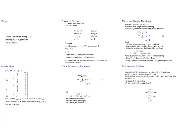
Quickly: Matrix View, Taking Dual. Matching, algebra, geometry. Facility Location.

Rules for School...

• r...”Rules for taking duals”

Canonical Form. Primal LP Dual LP max c ·x min yT b Ax ≤ b yT A ≥ c x ≥ 0 y ≥ 0 Standard: Ax ≤ b,maxcx,x ≥ 0 ↔ yT A ≥ c,minby,y ≥ 0. min ↔ max ≥↔≤ “inequalities” ↔ “nonnegative variables” “nonnegative variables” ↔ “inequalities” Another useful trick: Equality constraints. “equalities” ↔ “unrestricted variables.”

Maximum Weight Matching.

Bipartite Graph G = (V,E), w : E → Z. Find maximum weight perfect matching. Solution: xe indicates whether edge e is in matching. max∑

e

wexe ∀v : ∑

e=(u,v)

xe = 1 pv xe ≥ 0 Dual. Variable for each constraint. pv unrestricted. Constraint for each variable. Edge e, pu +pv ≥ we Objective function from right hand side. min∑v pv min∑v pv ∀e = (u,v) : pu +pv ≥ we Weak duality? Price function upper bounds matching. ∑e∈M wexe ≤ ∑e=(u,v)∈M pu +pv ≤ ∑v pu. Strong Duality? Same value solutions. Hungarian algorithm !!!

Matrix View.

xe variable for e = (u,v). xe rhs · ··· ··· 1 . . . . . . . . . . . . 1 pu · ··· 1 ··· 1 · ··· ··· 1 . . . . . . . . . . . . 1 · ··· ··· 1 pv · ··· 1 ··· 1 · ··· ··· 1 . . . . . . . . . . . . 1

• bj

· · we · Row equation: ∑e=(u,v) xe = 1. Row (dual) variable: pu. Column variable: xe. Column (dual) constraint: pu +pv ≥ 1. Exercise: objectives?

Complementary Slackness.

max∑

e

wexe ∀v : ∑

e=(u,v)

xe = 1 pv xe ≥ 0 Dual: min∑v pv ∀e = (u,v) : pu +pv ≥ we Complementary slackness: Only match on tight edges. Nonzero pu on matched u.

Multicommodity Flow.

Given G = (V,E), and capacity function c : E → Z, and pairs (s1,t1),...,(sk,tk) with demands d1,...,dk. Route Di flow for each si,ti pair, so every edge has ≤ µc(e) flow with minimum µ. variables: fp flow on path p. Pi -set of paths with endpoints si,ti. minµ ∀e : ∑

p∋e

fp ≤ µce ∀i : ∑

p∈Pi

fp = Di fp ≥ 0

SLIDE 2

Take the dual.

minµ ∀e : ∑

p∋e

fp ≤ µce ∀i : ∑

p∈Pi

fp = Di fp ≥ 0 Modify to make it ≥, which “go with min. And only constants on right hand side. minµ ∀e :µce − ∑

p∋e

fp ≥ 0 ∀i : ∑

p∈Pi

fp = Di fp ≥ 0

Dual.

minµ ∀e :µce − ∑

p∋e

fp ≥ 0 de ∀i : ∑

p∈Pi

fp = Di di fp ≥ 0 Introduce variable for each constraint. Introduce constraint for each var: µ → ∑e cede = 1. fp → ∀p ∈ Pi di −∑e∈p de ≤ 0. Objective: right hand sides. max∑i Didi max∑

i

Didi ∀p ∈ Pi :di ≤ ∑

e∈p

d(e)

∑

e

cede = 1 di - shortest si,ti path length. Toll problem! Weak duality: toll lower bounds routing. Strong Duality. Tight lower bound. First lecture. Or Experts. Complementary Slackness: only route on shortest paths

• nly have toll on congested edges.

Matrix View

fp variable for path e1,e2,...,ek. p connects si,ti. fp µ rhs · ··· ··· · . . . . . . . . . . . . . . . de1 · ···

• 1

··· ce1 . . . . . . . . . . . . . . . de2 · ···

• 1

··· ce2 . . . . . . . . . . . . . . . dek · ···

• 1

··· cek . . . . . . . . . . . . . . . di · · 1 · ··· Di

• bj

1 1 1 1 Row constraint: ceµ −∑p∋e fp ≥ 0. Row (dual) variable: de. Row constraint: ∑p∈Pi fp = Di. Row (dual) variable: di. Column variable: fp. Column (dual) constraint: di −∑e∈p de ≤ 0. Column variable: µ. Column (dual) constraint: ∑e d(e)c(e) = 1. Exercise: objectives?

Exponential size.

Multicommodity flow. minµ ∀e :µce − ∑

p∋e

fp ≥ 0 ∀i : ∑

p∈Pi

fp = di fp ≥ 0 Dual is. max∑

i

Didi ∀p ∈ Pi :di ≤ ∑

e∈p

d(e) Exponential sized programs? Answer 1: We solved anyway! Answer 2: Ellipsoid algorithm. Find violated constraint → poly time algorithm. Answer 3: there is polynomial sized formulation. Question: what is it?

Maximum matching and simplex.

y z x .3 .7 1 .3 .7 .3 .7 .3 .7 1 1 1 1 maxx +y +z x ≤ 1 x +z ≤ 1 a = 1 z +y ≤ 1 b = 1 y ≤ 1 x ≥ 0 y ≥ 0 z ≥ 0 c = 1

Blue constraints intersect. Blue constraints redundant. Blue constraints tight. Sum: x +2z +y.

x y z X X X X X X X +1 −1 +1 Augmenting Path. Via Gaussian Elimination!

Facility location

Set of facilities: F, opening cost fi for facility i Set of clients: D. dij - distance between i and j. (notation abuse: clients/facility confusion.) Triangle inequality: dij ≤ dik +dkj.

SLIDE 3

Facility Location

Linear program relaxation: “Decision Variables”. yi - facility i open? xij - client j assigned to facility i. min ∑

i∈F

yifi + ∑

i∈F,j∈D

xijdij ∀j ∈ D ∑

i∈F

xij ≥ 1 ∀i ∈ F,j ∈ D xij ≤ yi, xij,yi ≥ 0 Facility opening cost. Client Connnection cost. Must connect each client. Only connect to open facility.

Integer Solution?

min ∑

i∈F

yifi + ∑

i∈F,j∈D

xijdij ∀j ∈ D ∑

i∈F

xij ≥ 1 ∀i ∈ F,j ∈ D xij ≤ yi, xij,yi ≥ 0 facility client 1 xij = 1

2 edges.

yi = 1

2 edges.

Facility Cost: 3

2 Connection Cost: 3

Any one Facility: Facility Cost: 1 Client Cost: 3.7 Make it worse? Sure. Not as pretty!

Round solution?

min ∑

i∈F

yifi + ∑

i∈F,j∈D

xijdij ∀j ∈ D ∑

i∈F

xij ≥ 1 ∀i ∈ F,j ∈ D xij ≤ yi, xij,yi ≥ 0 Round independently? yi and xij separately? Assign to closed facility! Round xij and open facilities? Different clients force different facilities open. Any ideas? Use Dual!

The dual.

mincx,Ax ≥ b ↔ maxbx,yT A ≤ c. min ∑

i∈F

yifi + ∑

i∈F,j∈D

xijdij ∀j ∈ D ∑

i∈F

xij ≥ 1 ∀i ∈ F,j ∈ D xij ≤ yi, min ∑

i∈F

yifi+ ∑

i∈F,j∈D

xijdij ∀j ∈ D ∑

i∈F

xij ≥ 1 ; αj ∀i ∈ F,j ∈ D yi −xij ≥ 0 ; βij xij,yi ≥ 0 max∑

j

αj ∀i

∑

j∈D

βij ≤ fi ; yi ∀i ∈ F,j ∈ D αi −βij ≤ dij ; xij βij,αj ≥ 0

Interpretation of Dual?

min ∑

i∈F

yifi + ∑

i∈F,j∈D

xijdij ∀j ∈ D ∑

i∈F

xij ≥ 1 ∀i ∈ F,j ∈ D xij ≤ yi, xij,yi ≥ 0 max∑

j

αj ∀i ∈ F

∑

j∈D

βij ≤ fi ∀i ∈ F,j ∈ D αj −βij ≤ dij xij αj,βij ≤ 0 αj charge to client. maximize price paid by client to connect! Objective: ∑j αj total payment. Client j travels or pays to open facility i. Costs client dij to get to there. Savings is αj −dij. Willing to pay βij = αj −dij.

i

βij j j′

i′ βi′j βi′j′

αj αj′ Total payment to facility i at most fi before opening. Complementary slackness: xij ≥ 0 if and only if αj ≥ dij.

• nly assign client to “paid to” facilities.

Use Dual.

• 1. Find solution to primal, (x,y). and dual, (α,β).
• 2. For smallest (remaining) αj,

(a) Let Nj = {i : xij > 0}. (b) Open cheapest facility i in Nj. Every client j′ with Nj′ ∩Nj = / 0 assigned to i.

• 3. Removed assigned clients, goto 2.

SLIDE 4

Integral facility cost at most LP facility cost.

Claim: Total facility cost is at most ∑i fiyi.

• 2. For smallest (remaining) αj,

(a) Let Nj = {i : xij > 0}. (b) Open cheapest facility i in Nj. Every client j′ with Nj′ ∩Nj = / 0 assigned to i. fi j

xij ≤ yi

k Proof: Step 2 picks client j. fmin - min cost facility in Nj fmin ≤ fmin ·∑i∈Nj xij ≤ fmin ∑i∈Nj yi ≤ ∑i∈Nj yifi. For k used in Step 2. Nj ∩Nk = / 0 for j and k in step 2. → Any facility in ≤ 1 sum from step 2. → total step 2 facility cost is ∑i yifi.

Connection Cost.

• 2. For smallest (remaining) αj,

(a) Let Nj = {i : xij > 0}. (b) Open cheapest facility i in Nj. Every client j′ with Nj′ ∩Nj = / 0 assigned to i. Client j is directly connected. Clients j′ are indirectly connected. j j′ αj αj′ Connection Cost of j: ≤ αj. Connection Cost of j′: ≤ αj′ +αj +αj ≤ 3αj′. since αj ≤ αj′ Total connection cost: at most 3∑j′ αj ≤ 3 times Dual OPT. Previous Slide: Facility cost: ≤ primal “facility” cost ≤ Primal OPT. Total Cost: 4 OPT.

Twist on randomized rounding.

Client j: ∑i xij = 1, xij ≥ 0. Probability distribution! → Choose from distribution, xij, in step 2. Expected opening cost: ∑i∈Nj xijfi ≤ ∑i∈Nj yifi. and separate balls implies total ≤ ∑i yifi. Dj = ∑i xijdij Connection cost of primal for j. Expected connection cost j′ αj +αj′ +Dj. In step 2: pick in increasing order of αj +Dj. → Expected cost is (2αj′ +Dj′). Connection cost: 2∑j αj +∑j Dj. 2OPT(D) plus connection cost or primal. Total expected cost: Facility cost is at most facility cost of primal. Connection cost at most 2OPT + connection cost of prmal. → at most 3OPT.

Primal dual algorithm.

• 1. Feasible integer solution.
• 2. Feasible dual solution.
• 3. Cost of integer solution ≤ α times dual value.

Just did it. Used linear program. Faster? Typically. Begin with feasible dual. Raise dual variables until tight constraint. Set corresponding primal variable to an integer. Recall Dual: max∑

j

αj ∀i ∈ F

∑

j∈D

βij ≤ fi ∀i ∈ F,j ∈ D αj −βij ≤ dij αj,βij ≤ 0

Facility location primal dual.

Phase 1: 1. Initially αj,βij = 0.

• 2. Raise αj for every (unconnected) client.

When αj = dij for some i raise βij at same rate Why? Dual: αj −βij ≤ dij. Intution:Paying βij to open i. Stop when ∑i βij = fi. Why? Dual: ∑i βij ≤ fi Intution: facility paid for. Temporarily open i. Connect all tight ji clients j to i.

• 3. Continue until all clients connected.

Phase 2: Connect facilities that were paid by same client. Permanently open an independent set of facilities. For client j, connected facility i is opened. Good. Connected facility not open → exists client j′ paid i and connected to open facility. Connect j to j′’s open facility. β = .5 α = 1.5 Constraints for dual. ∑j βij ≤ fi αi −βij ≤ dij. Grow αj. αj = dij! Tight constraint: αj −βij ≤ dij. Grow βij (and αj). ∑j βij = fi for all facilities. Tight: ∑j βij ≤ fi LP Cost: ∑j αj = 4.5 Temporarily open all facilities. Assign Clients to “paid to” open facility. Connect facilities with client that pays both. Open independent set. Connect to “killer” client’s facility. Cost: 1 + 3.7 = 4.7. A bit more than the LP cost.

SLIDE 5

Analysis

Claim: Client only pays one facility. Independent set of facilities. Claim: Si - directly connected clients to open facility i. fi +∑j∈Si dij ≤ ∑j αj. Proof: fi = ∑j∈Si βij = ∑j∈Si αj −dij. Since directly connected: βij = αj −dij.

Analysis.

Claim: Client j is indirectly connected to i → dij ≤ 3αj. Directly connected to (temp open) i′ conflicts with i. exists j′ with αj′ ≥ dij′ and αj ≥ di′j′. When i′ opens, stops both αj and α′

j .

α′

j stopped no later (..maybe earlier..)

αj ≤ α′

j .

Total distance from j to i′. dij +dij′ +di′j′ ≤ 3αj j i′ i j′

Putting it together!

Claim: Client only pays one facility. Claim: Si - directly connected clients to open facility i. fi +∑j∈Si dij ≤ ∑j αj. Claim: Client j is indirectly connected to i → dij ≤ 3αj. Total Cost: direct clients dual (αj) pays for facility and own connections. plus no more than 3 times indirect client dual. Total Cost: 3 times dual. feasible dual upper bounds fractional (and integer) primal. 3 OPT. Fast! Cheap! Safe!

See you on Thursday.