X u a u a a matching. 3 3 3 0 0 1 dashed means matched. - - PowerPoint PPT Presentation

Comments on last lecture.

Easy to come up with several Nash for non-zero-sum games. Is the game framework only interesting in some infinite horizon? No. Minimize worst expected loss. Best defense. Any prior distribution on opponent. Best offense. Rational players should play this way! “Infinite horizon” is just an assumption of rationality.

Today

Finish Maximum Weight Matching Algorithm. Exact algorithm with dueling players. Multiplicative Weights Framework. Very general framework of toll/congestion algorithm.

Matching/Weighted Vertex Cover

Maximum Weight Matching. Given a bipartite graph, G = (U,V,E), with edge weights w : E → R, find a maximum weight matching. A matching is a set of edges where no two share an endpoint. Minimum Weight Cover. Given a bipartite graph, G = (U,V,E), with edge weights w : E → R, find an vertex cover function of minimum total value. A function p : V → R, where for all edges, e = (u,v) p(u)+p(v) ≥ w(e). Minimize ∑v∈U∪V p(u). Optimal solutions to both if for e ∈ M, w(e) = p(u)+p(v) (Defn: tight edge.) and perfect matching.

Maximum Weight Matching

Goal: perfect matching on tight edges. . . . . . . . . . ...

p(·) p(·)−δ p(·) p(·)+δ

Algorithm Start with empty matching, feasible cover function (p(·)) Add tight edges to matching. Use alt./aug. paths of tight edges. ”maximum matching algorithm.” No augmenting path. Cut, (S,T), in directed graph of tight edges! All edges across cut are not tight. (loose?) Nontight edges leaving cut, go from SU, TV. Lower prices in SU, raise prices in ST , all explored edges still tight, backward edges still feasible ... and get new tight edge! What’s delta? w(e) > p(u)+p(v) → δ = mine∈(SU×TV )w(e)−p(u)−p(v).

Some details/Runtime

Add 0 value edges, so that optimal solution contains perfect matching. Beginning “Matcher” Solution: M = {}. Feasible! Value = 0. Beginning “Coverer” Solution: p(u) = maximum incident edge for u ∈ U, 0 otherwise. Main Work: breadth first search from unmatched nodes finds cut. Update prices (find minimum delta.) Simple Implementation: Each bfs either augments or adds node to S in next cut. O(n) iterations per augmentation. O(n) augmentations. O(n2m) time.

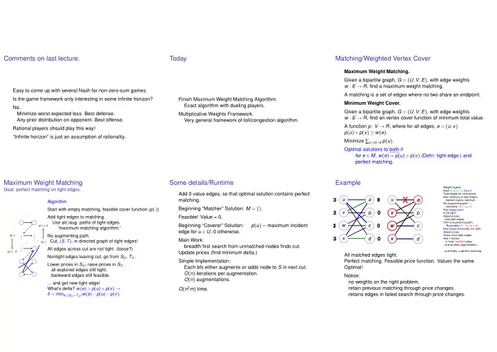
Example

u v w x a b c d 3 3 3 3 3 2 2 3 3 1 1 2 1 u v w x a b c d v w v w x a

X

Weight legend: black 1, green 2, blue 3 Tight edges for inital prices. Max matching in tight edges. dashed means matched. No augmenting path → reachable: S = {u,v} Blue edges soon to be tight! Adjust prices... new tight edges. Still no augmenting path. Reachable S = {v,w,x,a} Blue edges minimally non-tight. Adjust prices. Some more tight edges. And X shows a “new” nontight edge. ..and another augmentation... ..and finally: a perfect matching.

All matched edges tight. Perfect matching. Feasible price function. Values the same. Optimal! Notice: no weights on the right problem. retain previous matching through price changes. retains edges in failed search through price changes.

The multiplicative weights framework. Expert’s framework.

n experts. Every day, each offers a prediction. “Rain” or “Shine.” Whose advise do you follow? “The one who is correct most often.” Sort of. How well do you do?

Infallible expert.

One of the expert’s is infallible! Your strategy? Choose any expert that has not made a mistake! How long to find perfect expert? Maybe..never! Never see a mistake. Better model? How many mistakes could you make? Mistake Bound. (A) 1 (B) 2 (C) logn (D) n −1 Adversary designs setup to watch who you choose, and make that expert make a mistake. n −1!

Concept Alert.

Note. Adversary: makes you want to look bad. ”You could have done so well”... but you didn’t! ha..ha! Analysis of Algorithms: do as well as possible!

Back to mistake bound.

Infallible Experts. Alg: Choose one of the perfect experts. Mistake Bound: n −1 Lower bound: adversary argument. Upper bound: every mistake finds fallible expert. Better Algorithm? Making decision, not trying to find expert! Algorithm: Go with the majority of previously correct experts. What you would do anyway!

Alg 2: find majority of the perfect

How many mistakes could you make? (A) 1 (B) 2 (C) logn (D) n −1 At most logn! When alg makes a mistake, |“perfect” experts| drops by a factor of two. Initially n perfect experts mistake → ≤ n/2 perfect experts mistake → ≤ n/4 perfect experts . . . mistake → ≤ 1 perfect expert ≥ 1 perfect expert → at most logn mistakes!

Imperfect Experts

Goal? Do as well as the best expert!

• Algorithm. Suggestions?

Go with majority? Penalize inaccurate experts? Best expert is penalized the least.

• 1. Initially: wi = 1.
• 2. Predict with weighted majority of experts.
• 3. wi → wi/2 if wrong.

Analysis: weighted majority

• 1. Initially: wi = 1.
• 2. Predict with

weighted majority of experts.

• 3. wi → wi/2 if

wrong. Goal: Best expert makes m mistakes. Potential function: ∑i wi. Initially n. For best expert, b, wb ≥

1 2m .

Each mistake: total weight of incorrect experts reduced by −1? −2? factor of 1

2?

each incorrect expert weight multiplied by 1

2!

total weight decreases by factor of 1

2? factor of 3 4?

mistake → ≥ half weight with incorrect experts. Mistake → potential function decreased by 3

4.

We have 1 2m ≤ ∑

i

wi ≤ 3 4 M n.

where M is number of algorithm mistakes.

Analysis: continued.

1 2m ≤ ∑i wi ≤

3

4

M n. m - best expert mistakes M algorithm mistakes.

1 2m ≤

3

4

M n. Take log of both sides. −m ≤ −M log(4/3)+logn. Solve for M. M ≤ (m +logn)/log(4/3) ≤ 2.4(m +logn) Multiple by 1−ε for incorrect experts... (1−ε)m ≤

• 1− ε

2

M n. Massage... M ≤ 2(1+ε)m + 2lnn

ε

Approaches a factor of two of best expert performance!

Best Analysis?

Two experts: A,B Bad example? Which is worse? (A) A right on even, B right on odd. (B) A right first half of days, B right second Best expert peformance: T/2 mistakes. Pattern (A): T −1 mistakes. Factor of (almost) two worse!

Randomization!!!!

Better approach? Use? Randomization! That is, choose expert i with prob ∝ wi Bad example: A,B,A,B,A... After a bit, A and B make nearly the same number of mistakes. Choose each with approximately the same probabilty. Make a mistake around 1/2 of the time. Best expert makes T/2 mistakes. Rougly optimal!

Randomized analysis.

Some formulas: For ε ≤ 1,x ∈ [0,1], (1+ε)x ≤ (1+εx) (1−ε)x ≤ (1−εx) For ε ∈ [0, 1

2],

−ε −ε2 ≤ ln(1−ε) ≤ −ε ε −ε2 ≤ ln(1+ε) ≤ ε Proof Idea: ln(1+x) = x − x2

2 + x3 3 −···

Randomized algorithm

Losses in [0,1]. Expert i loses ℓt

i ∈ [0,1] in round t.

• 1. Initially wi = 1 for expert i.
• 2. Choose expert i with prob wi

W , W = ∑i wi.

• 3. wi ← wi(1−ε)ℓt

i

W(t) sum of wi at time t. W(0) = n Best expert, b, loses L∗ total. → W(T) ≥ wb ≥ (1−ε)L∗. Lt = ∑i

wiℓt

i

W expected loss of alg. in time t.

Claim: W(t +1) ≤ W(t)(1−εLt) Loss → weight loss. Proof: W(t +1) ≤ ∑

i

(1−εℓt

i )wi

= ∑

i

wi −ε∑

i

wiℓt

i

= ∑

i

wi

• 1−ε ∑i wiℓt

i

∑i wi

• =

W(t)(1−εLt)

Analysis

(1−ε)L∗ ≤ W(T) ≤ n ∏t(1−εLt) Take logs (L∗)ln(1−ε) ≤ lnn +∑ln(1−εLt) Use −ε −ε2 ≤ ln(1−ε) ≤ −ε −(L∗)(ε +ε2) ≤ lnn −ε ∑Lt And ∑t Lt ≤ (1+ε)L∗ + lnn

ε .

∑t Lt is total expected loss of algorithm. Within (1+ε) ish of the best expert! No factor of 2 loss!

Gains.

Why so negative? Each day, each expert gives gain in [0,1]. Multiplicative weights with (1+ε)gt

i .

G ≥ (1−ε)G∗ − logn ε where G∗ is payoff of best expert. Scaling: Not [0,1], say [0,ρ]. L ≤ (1+ε)L∗ + ρ logn ε

Summary: multiplicative weights.

Framework: n experts, each loses different amount every day. Perfect Expert: logn mistakes. Imperfect Expert: best makes m mistakes. Deterministic Strategy: 2(1+ε)m + logn

ε

Real numbered losses: Best loses L∗ total. Randomized Strategy: (1+ε)L∗ + logn

ε

Strategy: Choose proportional to weights multiply weight by (1−ε)loss. Multiplicative weights framework! Applications next!