Today Maximum Weight Matching. Integer Vertex Solution. Any vertex - PowerPoint PPT Presentation

Today Maximum Weight Matching. Integer Vertex Solution. Any “vertex” solution is integer! Bipartite Graph G = ( V , E ) , w : E → Z . Find maximum weight perfect matching. Linear programming feasible region: Polytope . Solution: x e indicates whether edge e is in matching. Dimension of space: number of variables. Vertex: intersection of d linearly independent constraints. max ∑ w e x e d “tight” constraints. e ∀ v : ∑ x e = 1 p v Approximation Algorithm. e =( u , v ) max ∑ w e x e x e ≥ 0 Facility Location. e Dual. ∀ v : ∑ x e = 1 p v Variable for each constraint. p v unrestricted. e =( u , v ) Constraint for each variable. Edge e , p u + p v ≥ w e x e ≥ 0 Objective function from right hand side. min ∑ v p v min ∑ v p v ∀ e = ( u , v ) : p u + p v ≥ w e Dimension: m Only 2 n of the form ∑ e x e = 1. Weak duality? Price function upper bounds matching. ∑ e ∈ M w e x e ≤ ∑ e =( u , v ) ∈ M p u + p v ≤ ∑ v p u . Must have m − 2 n tight constraints of form x e = 0. Throw away variables that are 0. Strong Duality? Same value solutions. Hungarian algorithm !!! Constraint matrix C with 2 n variables. 2 n rows. ..and so on. 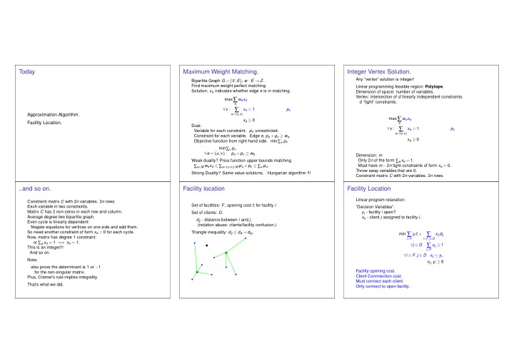Facility location Facility Location Linear program relaxation: Constraint matrix C with 2 n variables. 2 n rows. Set of facilities: F , opening cost f i for facility i Each variable in two constraints. “Decision Variables”. Matrix C has 2 non-zeros in each row and column. y i - facility i open? Set of clients: D . Average degree two bipartite graph. x ij - client j assigned to facility i . d ij - distance between i and j . Even cycle is linearly dependent: (notation abuse: clients/facility confusion.) Negate equations for vertices on one side and add them. So need another constraint of form x e = 0 for each cycle. Triangle inequality: d ij ≤ d ik + d kj . min ∑ y i f i + ∑ x ij d ij Now, matrix has degree 1 constraint: i ∈ F i ∈ F , j ∈ D or ∑ e x e = 1 = ⇒ x e = 1. ∀ j ∈ D ∑ x ij ≥ 1 This is an integer!!! i ∈ F And so on. ∀ i ∈ F , j ∈ D x ij ≤ y i , Note: x ij , y i ≥ 0 also prove the determinant is 1 or − 1 Facility opening cost. for the non-singular matrix. Client Connnection cost. Plus, Cramer’s rule implies integrality. Must connect each client. That’s what we did. Only connect to open facility.

Integer Solution? Round solution? The dual. min cx , Ax ≥ b ↔ max bx , y T A ≤ c . min ∑ y i f i + ∑ x ij d ij min ∑ y i f i + ∑ x ij d ij min ∑ y i f i + ∑ i ∈ F i ∈ F , j ∈ D x ij d ij i ∈ F i ∈ F , j ∈ D ∀ j ∈ D ∑ x ij ≥ 1 ∀ j ∈ D ∑ i ∈ F i ∈ F , j ∈ D x ij ≥ 1 ∀ j ∈ D ∑ i ∈ F x ij ≥ 1 i ∈ F ∀ i ∈ F , j ∈ D x ij ≤ y i , i ∈ F ∀ i ∈ F , j ∈ D x ij ≤ y i , x ij , y i ≥ 0 ∀ i ∈ F , j ∈ D x ij ≤ y i , x ij , y i ≥ 0 x ij = 1 Round independently? 2 edges. 1 min ∑ y i f i + ∑ max ∑ y i = 1 x ij d ij α j 2 edges. y i and x ij separately? Assign to closed facility! client i ∈ F i ∈ F , j ∈ D j Facility Cost: 3 2 Connection Cost: 3 Round x ij and open facilities? ∀ j ∈ D ∑ ∑ x ij ≥ 1 ; α j ∀ i β ij ≤ f i ; y i Any one Facility: Different clients force different facilities open. i ∈ F j ∈ D Facility Cost: 1 Client Cost: 3 . 7 facility Any ideas? ∀ i ∈ F , j ∈ D y i − x ij ≥ 0 ; β ij ∀ i ∈ F , j ∈ D α j − β ij ≤ d ij ; x ij Make it worse? Sure. Not as pretty! Use Dual! x ij , y i ≥ 0 β ij , α j ≥ 0 Interpretation of Dual? Use Dual. Integral facility cost at most LP facility cost. max ∑ α j min ∑ y i f i + ∑ x ij d ij j Claim: Total facility cost is at most ∑ i f i y i . i ∈ F i ∈ F , j ∈ D ∑ ∀ i ∈ F β ij ≤ f i ∀ j ∈ D ∑ x ij ≥ 1 2. For smallest (remaining) α j , j ∈ D i ∈ F (a) Let N j = { i : x ij > 0 } . ∀ i ∈ F , j ∈ D α j − β ij ≤ d ij 1. Find solution to primal, ( x , y ) . and dual, ( α , β ) . x ij ∀ i ∈ F , j ∈ D x ij ≤ y i , (b) Open cheapest facility i in N j . α j , β ij ≥ 0 Every client j ′ with N j ′ ∩ N j � = / 2. For smallest (remaining) α j , 0 assigned to i . x ij , y i ≥ 0 (a) Let N j = { i : x ij > 0 } . Proof: Step 2 picks client j . (b) Open cheapest facility i in N j . α j charge to client. Every client j ′ with N j ′ ∩ N j � = / f min - min cost facility in N j 0 assigned to i . maximize price paid by client to α j ′ f i f min ≤ f min · ∑ i ∈ N j x ij ≤ f min ∑ i ∈ N j y i ≤ ∑ i ∈ N j y i f i . connect! k x ij ≤ y i α j 3. Removed assigned clients, goto 2. j ′ Objective: ∑ j α j total payment. β ij For k used in Step 2. i ′ β i ′ j Client j travels or pays to open facility i . j N j ∩ N k = / 0 for j and k in step 2. Costs client d ij to get to there. i j β i ′ j ′ → Any facility in ≤ 1 sum from step 2. Savings is α j − d ij . → total step 2 facility cost is ≤ ∑ i y i f i . Willing to pay β ij = α j − d ij . Total payment to facility i at most f i before opening. Complementary slackness: x ij ≥ 0 if and only if α j ≥ d ij . only assign client to “paid to” facilities.

Connection Cost. Twist on randomized rounding. Primal dual algorithm. 1. Feasible integer solution. 2. Feasible dual solution. Client j : ∑ i x ij = 1, x ij ≥ 0. 2. For smallest (remaining) α j , 3. Cost of integer solution ≤ α times dual value. Probability distribution! → Choose from distribution, x ij , in step 2. (a) Let N j = { i : x ij > 0 } . Just did it. Used linear program. Faster? (b) Open cheapest facility i in N j . Expected opening cost: Every client j ′ with N j ′ ∩ N j � = / 0 assigned to i . ∑ i ∈ N j x ij f i ≤ ∑ i ∈ N j y i f i . Typically. (If dual is maximization.) Client j is directly connected. Clients j ′ are indirectly connected. and separate balls implies total ≤ ∑ i y i f i . Begin with feasible dual. Raise dual variables until tight constraint. D j = ∑ i x ij d ij Expected connection cost of primal for j . Set corresponding primal variable to an integer. Connection Cost of j : ≤ α j . Expected connection cost j ′ α j + α j ′ + D j . Connection Cost of j ′ : Recall Dual: ≤ α j ′ + α j + α j ≤ 3 α j ′ . In step 2: pick in increasing order of α j + D j . α j ′ since α j ≤ α j ′ → Expected cost is ≤ ( 2 α j ′ + D j ′ ) . α j j ′ max ∑ α j Total connection cost: Connection cost: 2 ∑ j α j + ∑ j D j . j 2 OPT ( D ) plus connection cost of primal. at most 3 ∑ j α j ≤ 3 times Dual OPT. j ∑ ∀ i ∈ F β ij ≤ f i Total expected cost: Previous Slide: Facility cost: j ∈ D Facility cost is at most facility cost of primal. ≤ primal “facility” cost ≤ Primal OPT. ∀ i ∈ F , j ∈ D α j − β ij ≤ d ij Connection cost at most 2 OPT + connection cost of prmal. Total Cost: 4 OPT. α j , β ij ≤ 0 → at most 3 OPT . Facility location primal dual. Analysis Phase 1: 1. Initially α j , β ij = 0. Constraints for dual. 2. Raise α j for every (unconnected) client. ∑ j β ij ≤ f i When α j = d ij for some i α i − β ij ≤ d ij . raise β ij at same rate Why? Dual: α j − β ij ≤ d ij . Grow α j . β = . 5 Intution:Paying β ij to open i . α j = d ij ! Claim: Client only pays one facility. Stop when ∑ i β ij = f i . Tight constraint: α j − β ij ≤ d ij . Why? Dual: ∑ i β ij ≤ f i Grow β ij (and α j ). Independent set of facilities. α = 1 . 5 Intution: facility paid for. ∑ j β ij = f i for all facilities. Claim: S i - directly connected clients to open facility i . Temporarily open i. Tight: ∑ j β ij ≤ f i f i + ∑ j ∈ S i d ij ≤ ∑ j α j . Connect all tight ji clients j to i . LP Cost: ∑ j α j = 4 . 5 Proof: 3. Continue until all clients connected. Temporarily open all facilities. f i = ∑ j ∈ S i β ij = ∑ j ∈ S i α j − d ij . Assign Clients to “paid to” open facility. Phase 2: Since directly connected: β ij = α j − d ij . Connect facilities with common client. Make “edge” between two facilities if paid by a common client. Open independent set. Permanently open an independent set of facilities in common client Connect to “killer” client’s facility. graph. Cost: 1 + 3.7 = 4.7. For client j , connected facility i is opened. Good. A bit more than the LP cost. Connected facility not open → exists client j ′ paid i and connected to open facility. Connect j to j ′ ’s open facility.

Analysis. Putting it together! Claim: Client only pays one facility. Claim: Client j is indirectly connected to i Claim: S i - directly connected clients to open facility i . → d ij ≤ 3 α j . f i + ∑ j ∈ S i d ij ≤ ∑ j α j . Check: if time. Claim: Client j is indirectly connected to i Directly connected to (temp open) i ′ conflicts with Won’t see you on Tuesday. → d ij ≤ 3 α j . i . Guest Speaker: Tselil Schramm. exists j ′ with α j ′ ≥ d ij ′ and α j ≥ d i ′ j ′ . Total Cost: When i ′ opens, stops both α j and α ′ j . direct clients dual ( α j ) pays for facility and own connections. Semidefinite Programming and Approximation. i ′ j i plus no more than 3 times indirect client dual. α j ′ stopped no later (..maybe earlier..) j ′ Total Cost: 3 times dual. α j ′ ≤ α j . Total distance from j to j ′ . feasible dual upper bounds fractional (and integer) primal. d ji ′ + d i ′ j ′ + d j ′ i ≤ 3 α j 3 OPT. Fast! Cheap! Safe!