Today Profit maximization. To pea or not to pea. 4$ for peas. 2$ - - PowerPoint PPT Presentation

Today

Continue Review: linear programming. Simplex and Matching. Taking Duals.

Profit maximization.

Plant Carrots or Peas? 2$ bushel of carrots. 4$ for peas. Carrots take 3 unit of water/bushel. Peas take 2 units of water/bushel. 100 units of water. Peas require 2 yards/bushel of sunny land. Carrots require 1 yard/bushel of shadyland. Garden has 60 yards of sunny land and 75 yards of shady land. To pea or not to pea, that is the question!

To pea or not to pea.

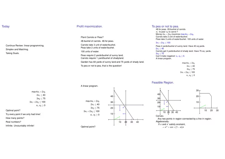
4$ for peas. 2$ bushel of carrots. x1- to pea! x2 to carrot ? Money 4x1 +2x2 maximize max4x1 +2x2. Carrots take 2 unit of water/bushel. Peas take 3 units of water/bushel. 100 units of water. 3x1 +2x2 ≤ 100 Peas 2 yards/bushel of sunny land. Have 40 sq yards. 2x1 ≤ 40 Carrots get 3 yards/bushel of shady land. Have 75 sq. yards. 3x2 ≤ 75 Can’t make negative! x1,x2 ≥ 0. A linear program. max4x1 +2x2 2x1 ≤ 40 3x2 ≤ 75 3x1 +2x2 ≤ 100 x1,x2 ≥ 0

max4x1 +2x2 2x1 ≤ 40 3x2 ≤ 75 3x1 +2x2 ≤ 100 x1,x2 ≥ 0 Optimal point? Try every point if we only had time! How many points? Real numbers?

• Infinite. Uncountably infinite!

A linear program. max4x1 +2x2 2x1 ≤ 40 3x2 ≤ 75 3x1 +2x2 ≤ 100 x1,x2 ≥ 0 10 20 30 40 10 20 30 40 Optimal point?

Feasible Region.

10 20 30 40 10 20 30 40 10 20 30 10 20 30 Convex. Any two points in region connected by a line in region. Algebraically: If x and x′ satisfy onstraint, → x′′ = αx +(1−α)x

10 20 30 10 20 30 Optimal at pointy part of feasible region! Vertex of region. Intersection of two of the constraints (lines in two dimensions)! Try every vertex! Choose best. O(m2) if m constraints and 2 variables. For n variables, m constraints, how many? nm? m

n

• ? n +m?

m

n

• Finite!!!!!!

Exponential in the number of variables. 10 20 30 10 20 30 max4x1 +2x2 3x1 ≤ 60 3x2 ≤ 75 3x1 +2x2 ≤ 100 x1,x2 ≥ 0

Simplex: Start at vertex. Move to better neighboring vertex. Until no better neighbor. This example. (0,0) objective 0. → (0,25) objective 50. → (16 2

3,25) objective 115 2 3

→ (20,20) objective 120. Duality: Add blue equations to get objective function? 1/3 times first plus second. Get 4x1 +2x2 ≤ 120. Every solution must satisfy this inequality! Objective value: 120. Can we do better? No! Dual problem: add equations to get best upper bound.

Duality.

maxx1 +8x2

x1 ≤ 4 x2 ≤ 3 x1 +2x2 ≤ 7 x1,x2 ≥ 0

One Solution: x1 = 1,x2 = 3. Value is 25. Best possible? For any solution. x1 ≤ 4 and x2 ≤ 3 .. ....so x1 +8x2 ≤ 4+8(3) = 28. Added equation 1 and 8 times equation 2 yields bound on objective.. Better solution? Better upper bound?

Duality.

maxx1 +8x2

x1 ≤ 4 x2 ≤ 3 x1 +2x2 ≤ 7 x1,x2 ≥ 0

Solution value: 25. Add equation 1 and 8 times equation 2 gives.. x1 +8x2 ≤ 4+24 = 28. Better way to add equations to get bound on function? Sure: 6 times equation 2 and 1 times equation 3. x1 +8x2 ≤ 6(3)+7 = 25. Thus, the value is at most 25. The upper bound is same as solution! Proof of optimality!

Duality:example

Idea: Add up positive linear combination of inequalities to “get” upper bound on optimization function. Will this always work? How to find best upper bound?

Duality: computing upper bound.

Best Upper Bound. Multiplier Inequality y1 x1 ≤ 4 y2 x2 ≤ 3 y3 x1 + 2x2 ≤ 7 Adding equations thusly... (y1 +y3)x1 +(y2 +2y3)x2 ≤ 4y1 +3y2 +7y3. The left hand side should “dominate” optimization function: If y1,y2,y3 ≥ 0 and y1 +y3 ≥ 1 and y2 +2y3 ≥ 8 then.. x1 +8x2 ≤ 4y1 +3y2 +7y3 Find best yi’s to minimize upper bound?

The dual, the dual, the dual.

Find best yi’s to minimize upper bound? Again: If you find y1,y2,y3 ≥ 0 and y1 +y3 ≥ 1 and y2 +2y3 ≥ 8 then.. x1 +8x2 ≤ 4y1 +3y2 +7y3

min 4y1 +3y2 +7y3 y1 +y3 ≥ 1 y2 +2y3 ≥ 8 y1,y2,y3 ≥ 0

A linear program. The Dual linear program. Primal: (x1,x2) = (1,3); Dual: (y1,y2,y3) = (0,6,1). Value of both is 25! Primal is optimal ... and dual is optimal!

The dual.

In general. Primal LP Dual LP max c ·x min yT b Ax ≤ b yT A ≥ c x ≥ 0 y ≥ 0 Theorem: If a linear program has a bounded value, then its dual is bounded and has the same value. Weak Duality: primal (P) ≤ dual (D) Feasible (x,y) P(x) = c ·x ≤ yT Ax ≤ yT b ·x = D(y). Strong Duality: next lecture.

Complementary Slackness

Primal LP Dual LP max c ·x min yT b Ax ≤ b yT A ≥ c x ≥ 0 y ≥ 0 Given A,b,c, and feasible solutions x and y. Solutions x and y are both optimal if and only if xi(ci −(yT A)i) = 0, and yj(bj −(Ax)j). xi(ci −(yT A)i) = 0 → ∑i(ci −(yT A)i)xi = cx −yT Ax → cx = yT Ax. yj(bj −(Ax)j) = 0 → ∑i yj(bj −(Ax)j) = yb −yT Ax → by = yT Ax. cx = by. If both are feasible, cx ≤ by, so must be optimal. In words: nonzero dual variables only for tight constraints!

Again: simplex

10 20 30 10 20 30 max4x1 +2x2 3x1 ≤ 60 3x2 ≤ 75 3x1 +2x2 ≤ 100 x1,x2 ≥ 0 Simplex: Start at vertex. Move to better neighboring vertex. Until no better neighbor. Duality: Add blue equations to get objective function? 1/3 times first plus second. Get 4x1 +2x2 ≤ 120. Every solution must satisfy this inequality! Geometrically and Complementary slackness: Add tight constraints to “dominate objective function.” Don’t add this equation! Shifts.

Example: review.

maxx1 +8x2 min 4y1 +3y2 +7y3 x1 ≤ 4 y1 +y3 ≥ 1 x2 ≤ 3 y2 +2y3 ≥ 8 x1 +2x2 ≤ 7 x1,x2 ≥ 0 y1,y2,y3 ≥ 0

“Matrix form” max[1,8]·[x1,x2] min[4,3,7]·[y1,y2,y3]   1 1 1 2   x1 x2

• ≤

  4 3 7   [y1,y2,y3]   1 1 1 2   ≥ 1 8

• [x1,x2] ≥ 0

[y1,y2,y3] ≥ 0

Matrix equations.

max[1,8]·[x1,x2] min[4,3,7]·[y1,y2,y3]   1 1 1 2   x1 x2

• ≤

  4 3 7   [y1,y2,y3]   1 1 1 2   ≥ 1 8

• [x1,x2] ≥ 0

[y1,y2,y3] ≥ 0 We can rewrite the above in matrix form. A =   1 1 1 2   c = [1,8]b = [4,3,7] The primal is Ax ≤ b,maxc ·x,x ≥ 0. The dual is yTA ≥ c,minb ·y,y ≥ 0.

Rules for School...

• r...”Rules for taking duals”

Standard: Ax ≤ b,maxcx,x ≥ 0 ↔ yTA ≥ c,minby,y ≥ 0. min ↔ max ≥↔≤ “inequalities” ↔ “nonnegative variables” “nonnegative variables” ↔ “inequalities” One more useful trick: Equality constraints. “equalities” ↔ “unrestricted variables.”

Maximum Weight Matching.

Bipartite Graph G = (V,E), w : E → Z. Find maximum weight perfect matching. Solution: xe indicates whether edge e is in matching. max∑

e

wexe ∀v : ∑

e=(u,v)

xe = 1 pv xe ≥ 0 Dual. Variable for each constraint. pv unrestricted. Constraint for each variable. Edge e, pu +pv ≥ we Objective function from right hand side. min∑v pv min∑v pv ∀e = (u,v) : pu +pv ≥ we Weak duality? Price function upper bounds matching. ∑e∈M wexe ≤ ∑e=(u,v)∈M pu +pv ≤ ∑v pu. Strong Duality? Same value solutions. Hungarian algorithm !!!

Complementary Slackness.

max∑

e

wexe ∀v : ∑

e=(u,v)

xe = 1 pv xe ≥ 0 Dual: min∑v pv ∀e = (u,v) : pu +pv ≥ we Complementary slackness: Only match on tight edges. Nonzero pu on matched u.

Multicommodity Flow.

Given G = (V,E), and capacity function c : E → Z, and pairs (s1,t1),...,(sk,tk) with demands d1,...,dk. Route Di flow for each si,ti pair, so every edge has ≤ µc(e) flow with minimum µ. variables: fp flow on path p. Pi -set of paths with endpoints si,ti. minµ ∀e : ∑

p∋e

fp ≤ µce ∀i : ∑

p∈Pi

fp = Di fp ≥ 0

Take the dual.

minµ ∀e : ∑

p∋e

fp ≤ µce ∀i : ∑

p∈Pi

fp = Di fp ≥ 0 Modify to make it ≥, which “go with min. And only constants on right hand side. minµ ∀e :µce − ∑

p∋e

fp ≥ 0 ∀i : ∑

p∈Pi

fp = Di fp ≥ 0

Dual.

minµ ∀e :µce − ∑

p∋e

fp ≥ 0 de ∀i : ∑

p∈Pi

fp = Di di fp ≥ 0 Introduce variable for each constraint. Introduce constraint for each var: µ → ∑e cede = 1. fp → ∀p ∈ Pi di −∑e∈p de ≤ 0. Objective: right hand sides. max∑i Didi max∑

i

Didi ∀p ∈ Pi :di ≤ ∑

e∈p

d(e)

∑

e

cede = 1 di - shortest si,ti path length. Toll problem! Weak duality: toll lower bounds routing. Strong Duality. Tight lower bound. First lecture. Or Experts. Complementary Slackness: only route on shortest paths

• nly have toll on congested edges.

Exponential size.

Multicommodity flow. minµ ∀e :µce − ∑

p∋e

fp ≥ 0 ∀i : ∑

p∈Pi

fp = di fp ≥ 0 Dual is. max∑

i

Didi ∀p ∈ Pi :di ≤ ∑

e∈p

d(e) Exponential sized programs? Answer 1: We solved anyway! Answer 2: Ellipsoid algorithm. Find violated constraint → poly time algorithm. Answer 3: there is polynomial sized formulation. Question: what is it?

Maximum matching and simplex.

y z x .3 .7 1 .3 .7 .3 .7 .3 .7 1 1 1 1 maxx +y +z x ≤ 1 x +z ≤ 1 a = 1 z +y ≤ 1 b = 1 y ≤ 1 x ≥ 0 y ≥ 0 z ≥ 0

Blue constraints intersect. Blue constraints redundant. Blue constraints tight. Sum: x +2z +y.

x y z X X X X X X X See you on Thursday.