Today CS 188: Artificial Intelligence Formalizing Learning Spring - - PDF document

1

CS 188: Artificial Intelligence

Spring 2006

Lecture 11: Decision Trees 2/21/2006

Dan Klein – UC Berkeley Many slides from either Stuart Russell or Andrew Moore

Today

Formalizing Learning

Consistency Simplicity

Decision Trees

Expressiveness Information Gain Overfitting

Inductive Learning (Science)

• Simplest form: learn a function from examples
• A target function: f
• Examples: input-output pairs (x, f(x))
• E.g. x is an email and f(x) is spam / ham
• E.g. x is a house and f(x) is its selling price
• Problem:
• Given a hypothesis space H
• Given a training set of examples xi
• Find a hypothesis h(x) such that h ~ f
• Includes:
• Classification (multinomial outputs)
• Regression (real outputs)
• How do perceptron and naïve Bayes fit in? (H, f, h, etc.)

Inductive Learning

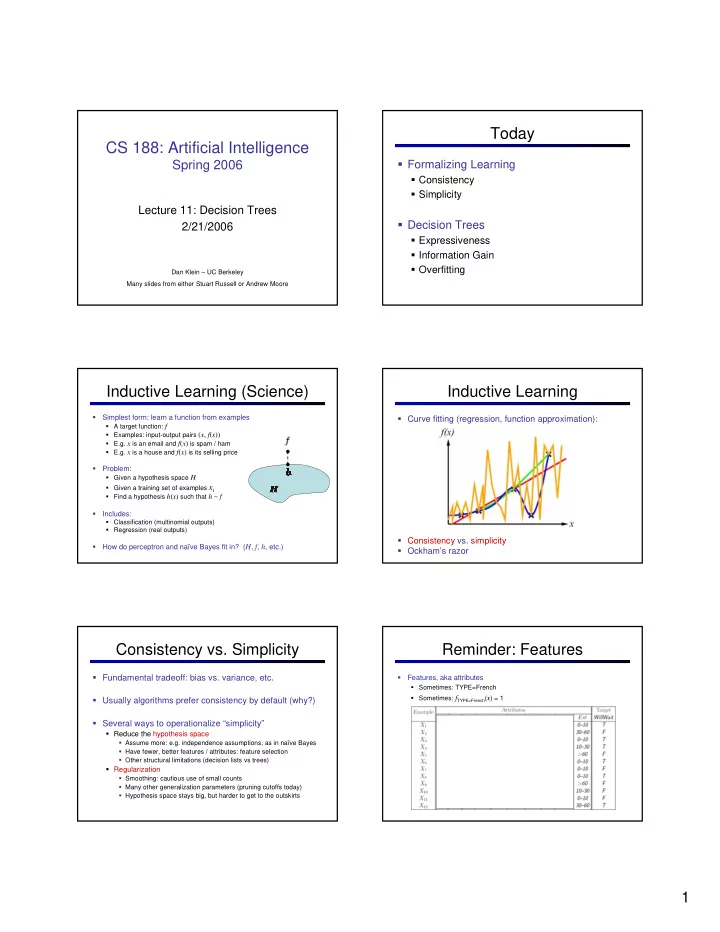
Curve fitting (regression, function approximation): Consistency vs. simplicity Ockham’s razor

Consistency vs. Simplicity

Fundamental tradeoff: bias vs. variance, etc. Usually algorithms prefer consistency by default (why?) Several ways to operationalize “simplicity”

Reduce the hypothesis space

Assume more: e.g. independence assumptions, as in naïve Bayes Have fewer, better features / attributes: feature selection Other structural limitations (decision lists vs trees)

Regularization

Smoothing: cautious use of small counts Many other generalization parameters (pruning cutoffs today) Hypothesis space stays big, but harder to get to the outskirts

Reminder: Features

• Features, aka attributes
• Sometimes: TYPE=French
• Sometimes: fTYPE=French(x) = 1

2

Decision Trees

Compact representation of a function:

Truth table Conditional probability table Regression values

True function

Realizable: in H

Expressiveness of DTs

Can express any function of the features However, we hope for compact trees

Comparison: Perceptrons

• What is the expressiveness of a perceptron over these features?
• DTs automatically conjoin features / attributes
• Features can have different effects in different branches of the tree!
• For a perceptron, a feature’s contribution is either positive or

negative

• If you want one feature’s effect to depend on another, you have to add a

new conjunction feature

• E.g. adding “PATRONS=full ∧ WAIT = 60” allows a perceptron to model

the interaction between the two atomic features

• Difference between modeling relative evidence weighting (NB) and

complex evidence interaction (DTs)

• Though if the interactions are too complex, may not find the DT greedily

Hypothesis Spaces

• How many distinct decision trees with n Boolean attributes?

= number of Boolean functions over n attributes = number of distinct truth tables with 2n rows = 2^(2n)

• E.g., with 6 Boolean attributes, there are

18,446,744,073,709,551,616 trees

• How many trees of depth 1 (decision stumps)?

= number of Boolean functions over 1 attribute = number of truth tables with 2 rows, times n = 4n

• E.g. with 6 Boolean attributes, there are 24 decision stumps
• More expressive hypothesis space:
• Increases chance that target function can be expressed (good)
• Increases number of hypotheses consistent with training set (bad, why?)
• Means we can get better predicitions (lower bias)
• But we may get worse predictions (higher variance)

Decision Tree Learning

• Aim: find a small tree consistent with the training examples
• Idea: (recursively) choose “most significant” attribute as root of

(sub)tree

Choosing an Attribute

Idea: a good attribute splits the examples into subsets that are (ideally) “all positive” or “all negative” So: we need a measure of how “good” a split is, even if the results aren’t perfectly separated out

3

Entropy and Information

Information answers questions

The more uncertain about the answer initially, the more information in the answer Scale: bits

Answer to Boolean question with prior <1/2, 1/2>? Answer to 4-way question with prior <1/4, 1/4, 1/4, 1/4>? Answer to 4-way question with prior <0, 0, 0, 1>? Answer to 3-way question with prior <1/2, 1/4, 1/4>?

A probability p is typical of:

A uniform distribution of size 1/p A code of length log 1/p

Entropy

General answer: if prior is <p1,…,pn>:

Information is the expected code length

Also called the entropy of the distribution

More uniform = higher entropy More values = higher entropy More peaked = lower entropy Rare values almost “don’t count”

1 bit 0 bits 0.5 bit

Information Gain

• Back to decision trees!
• For each split, compare entropy before and after
• Difference is the information gain
• Problem: there’s more than one distribution after split!
• Solution: use expected entropy, weighted by the number of examples
• Note: hidden problem here! Gain needs to be adjusted for large-domain

splits – why?

Next Step: Recurse

Now we need to keep growing the tree! Two branches are done (why?) What to do under “full”?

See what examples are there…

Example: Learned Tree

Decision tree learned from these 12 examples: Substantially simpler than “true” tree

A more complex hypothesis isn't justified by data

Also: it’s reasonable, but wrong

Example: Miles Per Gallon

40 Examples

mpg cylinders displacement horsepower weight acceleration modelyear maker good 4 low low low high 75to78 asia bad 6 medium medium medium medium 70to74 america bad 4 medium medium medium low 75to78 europe bad 8 high high high low 70to74 america bad 6 medium medium medium medium 70to74 america bad 4 low medium low medium 70to74 asia bad 4 low medium low low 70to74 asia bad 8 high high high low 75to78 america : : : : : : : : : : : : : : : : : : : : : : : : bad 8 high high high low 70to74 america good 8 high medium high high 79to83 america bad 8 high high high low 75to78 america good 4 low low low low 79to83 america bad 6 medium medium medium high 75to78 america good 4 medium low low low 79to83 america good 4 low low medium high 79to83 america bad 8 high high high low 70to74 america good 4 low medium low medium 75to78 europe bad 5 medium medium medium medium 75to78 europe

4

Find the First Split

Look at information gain for each attribute Note that each attribute is correlated with the target! What do we split on?

Result: Decision Stump Second Level

Final Tree

Reminder: Overfitting

Overfitting:

When you stop modeling the patterns in the training data (which generalize) And start modeling the noise (which doesn’t)

We had this before:

Naïve Bayes: needed to smooth Perceptron: didn’t really say what to do about it (stay tuned!)

MPG Training Error

The test set error is much worse than the training set error…

…why?

5

Consider this split

Significance of a Split

• Starting with:
• Three cars with 4 cylinders, from Asia, with medium HP
• 2 bad MPG
• 1 good MPG
• What do we expect from a three-way split?
• Maybe each example in its own subset?
• Maybe just what we saw in the last slide?
• Probably shouldn’t split if the counts are so small they could be due

to chance

• A chi-squared test can tell us how likely it is that deviations from a

perfect split are due to chance (details in the book)

• Each split will have a significance value, pCHANCE

Keeping it General

Pruning:

Build the full decision tree Begin at the bottom of the tree Delete splits in which pCHANCE > MaxPCHANCE Continue working upward until there are no more prunable nodes Note: some chance nodes may not get pruned because they were “redeemed” later

a b y 1 1 1 1 1 1

y = a XOR b

Pruning example

With MaxPCHANCE = 0.1:

Note the improved test set accuracy compared with the unpruned tree

Regularization

MaxPCHANCE is a regularization parameter Generally, set it using held

• ut data (as usual)

Small Trees Large Trees MaxPCHANCE Increasing Decreasing Accuracy High Bias High Variance Held-out / Test Training

Two Ways of Controlling Overfitting

Limit the hypothesis space

E.g. limit the max depth of trees Easier to analyze (coming up)

Regularize the hypothesis selection

E.g. chance cutoff Disprefer most of the hypotheses unless data is clear Usually done in practice

6

Learning Curves

Another important trend:

More data is better! The same learner will generally do better with more data (Except for cases where the target is absurdly simple)

Summary

Formalization of learning

Target function Hypothesis space Generalization

Decision Trees

Can encode any function Top-down learning (not perfect!) Information gain Bottom-up pruning to prevent overfitting