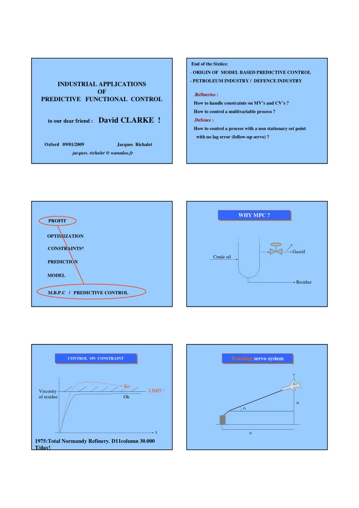
to our dear friend : David CLARKE ! .Defence : How to control a - PDF document

End of the Sixties: - ORIGIN OF MODEL BASED PREDICTIVE CONTROL - PETROLEUM INDUSTRY / DEFENCE INDUSTRY INDUSTRIAL APPLICATIONS OF .Refineries : PREDICTIVE FUNCTIONAL CONTROL How to handle constraints on MV’s and CV’s ? How to control a multivariable process ? to our dear friend : David CLARKE ! .Defence : How to control a process with a non stationary set point with no lag error (follow-up servo) ? Oxford 09/01/2009 Jacques Richalet jacques. richalet @ wanadoo.fr WHY MPC ? WHY MPC ? PROFIT OPTIMIZATION CONSTRAINTS* Gasoil Crude oil PREDICTION MODEL Residue M.B.P.C / PREDICTIVE CONTROL Tracking servo system CONTROL ON CONSTRAINT Tracking servo system CONTROL ON CONSTRAINT Ko LIMIT ! Viscosity of residue Ok H O t D 1975:Total Normandy Refinery. D11column 30.000 T/day!

….the past… NO LAG ERROR NO LAG ERROR 1968 : Basic principles of Predictive Control 1973 : 1st version of PFC/ IDCOM 1974 : 1st industrial applications of PFC/IDCOM Steam Generator/ Reactor/ Distillation P ε Τ = 0 ! 1978 : 1st contribution MPC “Automatica “ ( problems..!) X 1980-85 : HIECON with Set Point ( Houston) Target trajectory 1989 : Extension from PFC to PPC: Heading Parametric Predictive Control (control by reactor flow..) t 1998 :1st implementation of an MPC in the native library of a PLC : Modicon. Schneider-Electric.Momentum.Concept EXOTIC APPLICATIONS… FIRST INDUSTRIAL APPLICATIONS OF P.F.C. FIRST INDUSTRIAL APPLICATIONS OF P.F.C. METALLURGICAL INDUSTRIES North : Molde (Norway) DEFENCE � Coating lines aluminium � Mine hunter South : Plaza Huincul ( Patagonia-Argentina) � Thickness control - Roll eccentricity � Ariane 5 attitude control � Mono-multi-stands Rolling mills East : Hokaido ( Japan) � Missile autopilot � Continuous casting (slab) � Laser guided missile (t=62 microsecond…) � Push-ovens West : Mobile ( USA.DEGUSSA) � Gun turrets � Coke furnace � Radar antennas High : Eiffel Tower elevator ! � Hot/cold/Thin rolling mills � Infra Red camera � Steam generators � High speed Infra Red Space : European Space Agency : Mars project bioreactors ( 2029 !) Level, temperature, pressure……; � Missile launch � Camera mount Depth : Mine hunter boat � Radar antennas MISCELLANEOUS (Chem reactors and Speed : Temperature cabin ( TGV : 574.8 km/h W.record ) � Laser mirror distillation excluded) � Tank turret (T. 55) � s ) Fast : Laser guided bomb ( Tsampling : 65 � Mine sweeper auto-pilot � Bioreactor Melissa ESA � Aircraft carrier auto-pilot � Plastic extrusion robot (high speed) Slow : River dam level ( Tsampling : 1 hour) � Temperature control of gas furnace � Temperature control of TGV train carriage Ecology: Diester from colza AUTOMOTIVE � River dam level control (T=1 hour ) � Gear box test bench Animal : Dog food pellet dryer � Powder milk dryer � Dynamic test bench engine � Electric furnace brazing etc…. Plants : Greenhouses � Fuel injection � Idle fuel injection etc… � Clutch antistroke FEATURES � Gear box (tank) � Hybrid car (electric-fuel) …the oldest MBPC… 1968 � Air conditioning A “few” thousand applications in many fields AT WHAT LEVEL DO WE OPERATE ? N Histogram 2 Back to Basics: OFF • Level 0 : Ancillary processes e.g: FRC/ Pid SPEC 1.5 (the valve is the nightmare of control !) • Level 1 : Dynamic control with constraints 1 • Level 2 : Optimization of working conditions • Level 3 : Production planning Sigma 1 0.5 .Level N is operative if level N-1 works well…! Q1 QUALITY . »There are no technical problems, but only technical 0 0 50 100 150 200 250 300 350 400 450 aspects of economic problems … »

N Histogram N Histogram LEVEL 0 / LEVEL 1 LEVEL 0 / LEVEL 1 2 2 Sigma 1 -- Sigma 2 Sigma 1 -- Sigma 2 Sigma 2 Sigma 2 LEVEL 2 OFF OFF Q1 -- Q2 SPEC SPEC 1.5 1.5 1 1 Sigma 1 Sigma 1 0.5 0.5 Q1 QUALITY Q2 Q1 QUALITY 0 0 0 50 100 150 200 250 300 350 400 450 0 50 100 150 200 250 300 350 400 450 « SQUEEZE AND SHIFT » 4 BASIC PRINCIPLES OF PFC : J. PIAGET 4 BASIC PRINCIPLES OF PFC : J. PIAGET COST FUNCTION N Histogram LEVEL 0 / LEVEL 1 2 Sigma 1 -- Sigma 2 – Operating Image - Internal independant Model Sigma 2 LEVEL 2 OFF Q1 -- Q2 SPEC W2 1.5 – Target – Sub Target – Reference Trajectory DELTA COST (W2-W1) W1 1 – Action – Solver. Functional basis Structured future MV Sigma 1 0.5 – Comparison : – Predicted / Actual – Error compensator Q2 Q1 QUALITY 0 0 50 100 150 200 250 300 350 400 450 • Natural Control : “You would not drive your car using a PID scheme” TARGETED PERFORMANCES STRATEGY… . Control « all » types of processes: time delay, unstable, non-minimum phase, some non-linear . Control of industrial processes : PI(D) ? . Handles all constraints on the MV and on internal but PID cannot solve all control problems, variables of the process CV. but any candidate controller should « look like a PId »: . No lag error on dynamic set points with no integrator Industrial settings: EASY TO UNDERSTAND, TO IMPLEMENT, TO TUNE . Transparent and Cascade Control with transfer of constraints from inner loop to outer controller (« Back Calculation ») .. consistent with floor instrumentists’ habits . True feed-forward so: . Split-range control with different dynamics (reactors!) . Tuning parameters should have a clear, physical interpretation. . Control with 2 cooperative MV’s, e.g., big valve / small . Elementary mathematics. valve . No explicit integrator in the loop. . Extendable to 2 MV/ 2 CV….. . No matrix calculation. . Dual control: total elimination of harmonic disturbances . No quadratic minimization on-line. . Full Robustness analysis: easy trade-off , . No iterative computation on-line. . Immediate tuning / Open technology . Open technology…

2 T Y P E S O F M O D E L S n Future TRBF Past REFERENCE REFERENCE C(n+H) ε (n+H) TRAJECTORY TRAJECTORY perturbation perturbation Set point Reference Predicted output y ref trajectory y P ∆ + + ε (n) e Process sp e Process sp + + Process output y P sm sm Model Model ∆ M Re-aligned Model Independent Model Model output H H 1 H 2 y M Independent models are selected: Coïncidence horizon . Input /Output models valid for all math. structures MV Manipulated variable MV i . No permanent errors in steady-state modes! ( never mix process variables with model parameters..) Prediction horizon Solver Why structuring the future MV? • Determing all future MVs is of little benefit: • The future MV is projected on a Functional Basis: – many projects lead to the same future behaviour – e.g. Taylor expansion / polynomials • (low-pass process) • Thus, the MV is restricted a priori and not damped • Computation time increases ( PLC !) afterwards…. • Introduction of a damping term on the speed • MV(n+i) = ☞ j. Uj(i) Σ of the MV a priori is difficult to tune ! • U0(i) = 1, U1(i) = i U2(i)= i 2 etc … • Projection on « Eigen » functions of linear • Find the ☞ j such that: dynamic processes insures no lag error on – At a finite number of points, the predicted model output coincides with the desired reference trajectory dynamic set points • (i.e., coincidence points) OPEN LOOP ClOSED LOOP WITH CONSTRAINT 140 140 MV CONSTRAINT 120 120 SETPOINT MV 100 100 80 80 CV h=125 60 − − − − CLTR DESIRED =410 − − − − exp( 20 ).(1 15 ) s s CV = = 60 = = H s ( ) + + + + + + + + + + + + CLTR ACTUAL =424 (1 25 )(1 s 55 )(1 80 ) s s 40 40 dCV 20 20 0 0 -20 0 100 200 300 400 500 600 700 800 900 0 100 200 300 400 500 600 700 800 900 time

REFERENCE TRAJECTORY at ti=20 REFERENCE TRAJECTORY at ti=60 140 140 MV MV 120 120 Setpoint=100 Setpoint=100 100 100 80 80 60 60 REF TRAJ.(green) REF TRAJ.(green) CV PREDICTED(black) CV PREDICTED(black) 40 40 CV PASSED(red) CV PASSED(red) 20 20 tinit=20 tinit=60 0 0 -20 -20 100 200 300 400 500 600 700 800 900 100 200 300 400 500 600 700 800 900 REFERENCE TRAJECTORY at ti=100 REFERENCE TRAJECTORY at ti=150 140 140 MV MV 120 120 Setpoint=100 Setpoint=100 100 100 80 80 60 60 REF TRAJ.(green) REF TRAJ.(green) CV PREDICTED(black) CV PREDICTED(black) tinit=150 40 40 CV PASSED(red) CV PASSED(red) 20 20 tinit=100 0 0 -20 -20 100 200 300 400 500 600 700 800 900 100 200 300 400 500 600 700 800 900 REFERENCE TRAJECTORY at ti=200 REFERENCE TRAJECTORY at ti=300 140 140 MV MV 120 120 Setpoint=100 Setpoint=100 100 100 tinit=300 80 80 tinit=200 60 60 REF TRAJ.(green) REF TRAJ.(green) CV PREDICTED(black) CV PREDICTED(black) 40 40 CV PASSED(red) CV PASSED(red) 20 20 0 0 -20 -20 100 200 300 400 500 600 700 800 900 100 200 300 400 500 600 700 800 900